The METviewer database and display system provides a flexible and interactive interface to ingest and visualize the statistical output of MET. In this tutorial, we loaded the MET outputs for each of the 3 supported case into separate databases named mv_derecho, mv_sandy, and mv_snow, which required running METviewer separately for each case by pointing to the specific ${CASE_DIR} directory. While sometimes it is desirable for each case to have its own database within a single METviewer instance, sometimes it is advantageous to load MET output from multiple cases into the same METviewer instance. For example, if a user had multiple WRF configurations they were running over one case, and they wanted to track the performance of the different configurations, they could load both case outputs into METviewer and analyze them together. The customization example below demonstrates how to load MET output from multiple cases into a METviewer database.
Load MET output from multiple cases into a METviewer database
In this example, we will execute a series of three steps: 1) reorganize the MET output from multiple cases to live under a new, top-level directory, 2) launch the METviewer container, using a modified Docker compose YML file, and 3) execute a modified METviewer load script to load the data into the desired database. For example purposes, we will have two cases: sandy (supplied, unmodified sandy case from the tutorial) and sandy_mp8 (modified sandy case to use Thompson microphysics, option 8); these instructions will only focus on the METviewer steps, assuming the cases have been run through the step to execute MET and create verification output.
Step 1: Reorganize the MET output
In order to load MET output from multiple cases in a METviewer database, the output must be rearranged from its original directory structure (e.g., $PROJ_DIR/sandy) to live under a new, top-level cases directory (e.g., $PROJ_DIR/cases/sandy). In addition, a new, shared metviewer/mysql directory must also be created.
mkdir -p $PROJ_DIR/metviewer/mysql
Once the directories are created, the MET output needs to be copied from the original location to the new location.
cp -r $PROJ_DIR/sandy_mp8/metprd/* $PROJ_DIR/cases/sandy_mp8
Step 2: Launch the METviewer container
In order to visualize the MET output from multiple cases using the METviewer database and display system, you first need to launch the METviewer container. These modified YML files differ from the original files used in the supplied cases by modifying the volume mounts to no longer be case-specific (i.e., use $CASE_DIR).
| FOR NON-AWS: | FOR AWS: |
|---|---|
|
|
|
Step 3: Load MET output into the database(s)
The MET output then needs to be loaded into the MySQL database for querying and plotting by METviewer by executing the load script (metv_load_cases.ksh), which requires three command line arguments: 1) name of database to load MET output (e.g., mv_cases), 2) path in Docker space where the case data will be mapped, which will be /data/{name of case directory used in Step 1}, and 3) whether you want a new database to load MET output into (YES) or load MET output into a pre-existing database (NO). In this example, where we have sandy and sandy_mp8 output, the following commands would be issued:
docker exec -it metviewer /scripts/common/metv_load_cases.ksh mv_cases /data/sandy_mp8 NO
The METviewer GUI can then be accessed with the following URL copied and pasted into your web browser:
Note, if you are running on AWS, run the following commands to reconfigure METviewer with your current IP address and restart the web service:
|
docker exec -it metviewer /bin/bash
/scripts/common/reset_metv_url.ksh exit |
The METviewer GUI can then be accessed with the following URL copied and pasted into your web browser (where IPV4_public_IP is your IPV4Public IP from the AWS “Active Instances” web page):
http://IPV4_public_IP/metviewer/metviewer1.jsp
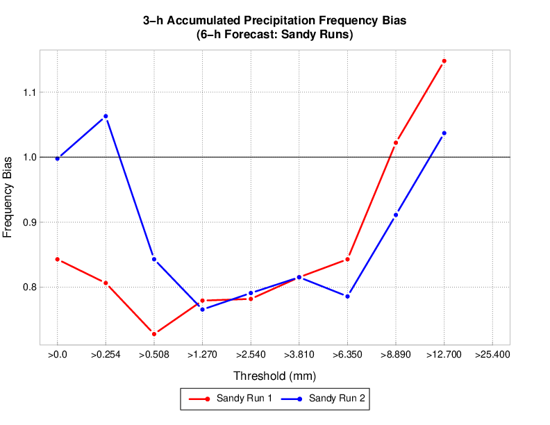
These commands would load sandy and sandy_mp8 MET output into the mv_cases database. An example METviewer plot using sandy sandy_mp8 MET output is shown below (click here for XML used to create the plot).