Verification Statistics for Continuous Forecasts
The nature of continuous forecast verification is a direct comparison of the forecast and observed values and measurement of the relationship of those two values over the real number range. We can easily infer that the scalar statistics and skill scores used for these kinds of forecasts will be different from those used for binary and multi-categorical forecasts. In fact many of the statistics that are used as “introductory statistics” are derived for continuous verification along the real number range, as continuous verification is a natural way we look at forecasts (i.e., how close or far the forecast and observed values are from each other).
Mean Errors
The simplest continuous measure is the mean error (ME), which is the average difference between two groups of data. So when you see “error” it is simply a measure of a difference. ME is calculated as
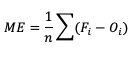
ME can range over the real numbers and has the obvious advantage of providing immediate insight into how far away, on average, the forecast values are from their corresponding observations. It is extremely easy to calculate, with a perfect forecast (i.e., a forecast that exactly corresponds to the observations) characterized by an ME of 0. ME serves as an important measurement of arithmetic bias. As a measure of bias, ME does not include a method for compensating for the magnitude of the differences between the forecast-observation pairs, and a forecast that has compensating errors could receive a mean error of 0. Essentially, ME provides an indication of whether a forecast has errors that - on average - are centered on zero; or if it is overforecasting or underforecasting on average. Consider the following scenario for wind speed forecasts at the same location for four different times:
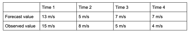
You’ll find the ME computed with these data equals 0, even though the difference between forecast and observation values for all of the times are non-zero. That’s because those errors that are positive (the forecast was greater than the observed value) are exactly negated by those errors that are negative (the forecast was less than the observed value). As noted earlier, ME is a good measure of bias; however, it is not a measure of accuracy.
This ability to effectively “hide” errors calls for a more robust error calculation to understand the forecasts’ accuracy. To that end, a few additional choices for measuring error are available.
Mean absolute error (MAE), while similar to ME, examines the absolute values of the errors, which are summed and averaged, providing a measure of accuracy as opposed to bias. Examining the absolute values of the errors restricts MAE’s range from zero to positive infinity, with a perfect score of zero:
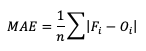
MAE also differs from ME in that it measures forecast accuracy, while ME measures bias. MAE provides a summary of the average magnitudes of the errors, but does not provide information about the direction (positive or negative) of the error magnitude.
Mean Squared Error (MSE) is another statistic focused on the characteristics of the forecast errors that measures forecast accuracy. In particular, MSE summarizes the squared differences between the forecast and observed values:
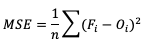
This measure has the same limits and perfect score as MAE, but squaring the differences does more than remove the sign of the differences: by squaring the error values, differences greater than one are penalized more severely than those that are less than one, with the penalty increasing at a squared rate. Using MSE, a forecast that over-forecasts temperature by two degrees from the observed value consistently over six time steps will have a smaller MSE than a forecast that over-forecasts temperature from the observed value by three degrees for three time steps and matched the observed value for the remaining three time steps.
The final error statistic to discuss is Root Mean Squared Error (RMSE). One of the most familiar statistical measures, RMSE is simply the square root of MSE, and has the same units as the forecasts and observations, providing an average error with a square-weight:
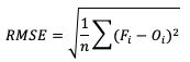
Similar to MSE, RMSE penalizes larger error magnitudes than smaller ones, and like MSE, RMSE provides no information on the sign (positive or negative) of the errors. It has the same range of values as MSE and a perfect forecast score would be an RMSE of zero. See how to use these statistics in METplus!
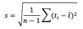
Standard Deviations
Unlike the family of mean error statistics, standard deviation focuses more on the individual groups of value sources; namely, the forecasts and observations. Standard deviations are a measure of how the variability of the values in a dataset differs from the average of their respective group. So keep in mind the general equation provided below can be applied to both observations and forecasts (and in some cases it may be meaningful to compare the standard deviation of the forecasts to the standard deviation of the observations):
See how to use this statistic in METplus!
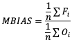
Multiplicative Bias
Like some of the other verification statistics for continuous forecasts, multiplicative bias (MBIAS) measures the ratio of the average forecast to the average observation. MBIAS is the ratio between these two averages, calculated using the following formula and has a range of all real numbers:
MBIAS has some of the same drawbacks as ME. In particular, MBIAS does not indicate the magnitudes of the forecast errors, which allows a perfect score of 1 to be achieved if the forecast errors compensate for each other (see the example for ME above for more information). It is recommended that any variable fields that utilize MBIAS contain all the same value signs (e.g. positive or negative) as mixing value signs together (for example, temperatures) would result in strange or unusable MBIAS results that included even more value compensation. See how to use this statistic in METplus!
Correlation Coefficients (Pearson, Spearman Rank, and Kendall’s Tau)
Because continuous forecasts and observations exist on the same real value spectrum, measurements of the linear association of the forecast-observation pairs create a vital foundation for verification statistics. Three measures of correlation (Pearson, Spearman Rank, and Kendall's Tau) measure this relationship in different ways.
Beginning with Pearson correlation coefficient, PR_CORR, the linear association of the forecast-observation pairs is measured using a sample covariance (e.g. the summed squared anomalies of two groups) and dividing by the product of the same two group’s standard deviations. In forecast verification, these two groups are the forecast and observation datasets and appear as
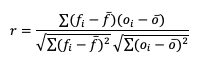
with r as the typical notation for the PR_CORR outside of METplus. From a visual perspective, PR_CORR measures the closeness of pairs of points, (i.e., representing the forecast and corresponding observation values) corresponding to a diagonal line. More generally these scatter plots can suggest the apparent relationship of any two variable fields, but for the purpose of this tutorial we will stay focused on the forecast-observation comparison. PR_CORR can range from negative one to positive one with either extreme of the range representing a perfect positive or negative linear association between the forecasts and observations. The PR_CORR remains sensitive to outliers and can produce a good correlation value for a poor forecast if that forecast has compensative errors.
Another way to estimate the linear association between forecasts and their corresponding observations involves ranking the forecast values when compared to the forecast group’s total range, do the same for the observation group, and then compute the correlation values. Spearman Rank correlation coefficient (SP_CORR) takes this approach while utilizing the same equation as PR_CORR. Because the rank values of both the forecast and observation datasets used to calculate SP_CORR are restricted to the integer values of 1 to n (the total number of matched forecast-observation pairs), the equation of SP_CORR can be simplified to
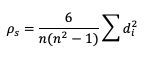
where di denotes the difference in ranking between the pair of datafields.
What does ranking of matched pairs look like with actual data? Let’s use the following scenario of rainfall forecasts and the observed rainfall over a five hour period for a set location:
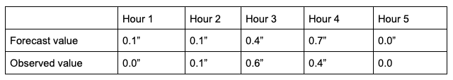
Using a ranking system for the datasets where 0.0” is assigned 1 and everything greater than that value is assigned a value that is integer-based, monotonically increasing by 1, the data table above would be transformed into the following ranks:
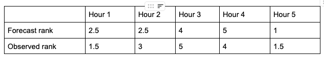
It is important that the forecast-observation pairs stay paired together, even when transformed into their rank values. Note the case when there is a tie in the ranks (i.e. a value appears more than once), all of the values receive the same average rank, keeping the total average rank for the number of values (in this scenario, five) consistent with the SP_CORR equation assumption. The next step is calculating the differences between the forecast ranks and the observed ranks, squaring the differences and summing them. After that, apply the rest of the equation and you should find ρ_s =0.825, a strong correlation value.
The Kendall’s Tau statistic (𝝉) is a variation on the SP_CORR equation ranking method. While all of the variable field values are ranked as was the case with SP_CORR, it’s the relationship between a pair of ranks and the pairs of ranks that follow, rather than the ranks within a given pair, that constitute 𝝉. To better understand, let’s first look at the equation for 𝝉:
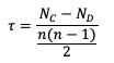
In the equation, N_C is a count of the concordant pairs, and N_D is a count of the discordant pairs. Simply put, a concordant pair is when a reference pair has rank values that are both larger or both smaller than a comparison pair. For example, consider the two pairs (3, 5) and (6, 8). Regardless of which pair is treated as the reference pair, the comparison pair will have both of the larger rank values (the case where (3, 5) is the reference pair) or both of the smaller rank values (the case where (6, 8) is the reference pair). A concordant pair is the complement to this: each pair in the comparison has one value that is bigger and one that is smaller. In the case of (3, 5) and (6, 2) the comparisons are considered discordant. In the case where the compared pairs are identical, there are multiple methods to choose: N_C and N_D can be incremented by ½ each, the tie can be ignored, or the tie can be penalized. For simplicity in counting, it is recommended to arrange one of the datasets in ascending or descending order (being careful to keep the matched pairs together) so that fewer comparisons need to be made.
To show how 𝝉 is calculated, let’s return to the previous example used to calculate SP_CORR. Because we’re using the same rainfall values, the rankings of those values will also be the same. For the simplicity of counting concordant and discordant pairs, the forecast ranks have been arranged in increasing order (which explains why Hour 5 is now proceeding Hour 1):
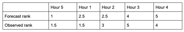
From this small change in the ordering, we see that two of the observed ranks do not increase (going from left to right): between Hour 5 and Hour 1 (they match at 1.5), and between Hour 3 and Hour 4 (5 compared to 4). Additionally, the forecast ranks between Hour 1 and Hour 2 do not increase (they match). In order to account for these ties, a “penalty” will be calculated using the following equation:
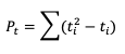
Where ti is the number of ranks that are involved in a given tie. Because both the forecast and observed ranks have a tie of two ranks, both will receive a Pt penalty of 2. As a result of this new handling of ties, an alternate form of 𝝉 sometimes referred to as 𝝉b must be used:
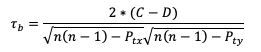
Using this slightly modified equation, we find a 𝝉b value of 0.56. As 𝝉 has the same range as SP_CORR (-1 to 1), a value of 0.56 shows some positive correlation between the two datasets. See how to use these statistics in METplus!
Anomaly Correlation
While similar to the traditional correlation coefficient, anomaly correlation is a somewhat different formulation: rather than directly comparing the pairs of forecast and observation values relative to the respective group averages, as is the case in PR_CORR, anomaly correlation is a measure of the deviations of forecast and observation values from climatological averages. Utilizing this third independent dataset for comparisons highlights any pattern of departures from the climatology, a correspondence of the forecast anomalies to the observed anomalies.
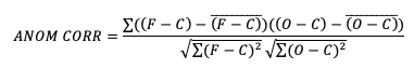
There are two widely used versions of anomaly correlation. The first is the centered anomaly correlation, which includes the mean error relative to the climatology. This version is calculated using
If it is not desirable to include the errors, the uncentered anomaly correlation is the better choice:
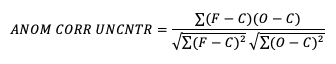
While there is an added effort required to find the matching climatology reference dataset for this statistic, it remains a highly resourceful statistic to use, especially with spatial verification, and is commonly used in operational forecasting centers. Anomaly correlation has a range from -1 to 1. See how to use this statistic in METplus!