METplus Practical Session Guide (Version 5.0) | Continuous Forecasts > METplus Examples of Continuous Forecast Verification

The following two examples show a generalized method for calculating continuous statistics: one for a MET-only usage, and the same example but utilizing METplus wrappers. These examples are not meant to be completely reproducible by a user: no input data is provided, commands to run the various tools are not given, etc. Instead, they serve as a general guide of one possible setup among many that produce continuous statistics.

If you are interested in reproducible, step-by-step examples of running the various tools of METplus, you are strongly encouraged to review the METplus online tutorial that follows this statistical tutorial, where data is made available to reproduce the guided examples.

In order to better understand the delineation between METplus, MET, and METplus wrappers which are used frequently throughout this tutorial but are NOT interchangeable, the following definitions are provided for clarity:

• METplus is best visualized as an overarching framework with individual components. It encapsulates all of the repositories: MET, METplus wrappers, METdataio, METcalcpy, and METplotpy.
• MET serves as the core statistical component that ingests the provided fields and commands to compute user-requested statistics and diagnostics.
• METplus wrappers is a suite of Python wrappers that provide low-level automation of MET tools and plotting capability. While there are examples of calling METplus wrappers without any underlying MET usage, these are the exception rather than the rule.

MET Example of Continuous Forecast Verification

Here is an example that demonstrates deterministic forecast verification in MET.

For this example, let’s examine two tools, PCP-Combine and Grid-Stat. Assume we wanted to verify a 6 hour period of precipitation forecasts over the continental United States. Using these tools, we will first combine the forecast files, which are hourly forecasts, into a 6 hour summation file with PCP-Combine. Then we will use Grid-Stat to place both datasets on the same verification grid and let MET calculate the continuous statistics available in the CNT line type. Starting with PCP-Combine, we need to understand what the desired output is first to know how to properly run the tool from the command line, as PCP-Combine does not use a configuration file. As stated previously, this scenario assumes the precipitation forecasts are hourly files and need to match the 6 hour observation file time summation. Of the four commands available in PCP-Combine, two seem to provide potential paths forward: sum and add.

While there are multiple methods that may work to successfully summarize the forecast files from these two commands, let’s assume that our forecast data files contain a time reference variable that is not CF-compliant {link to CF compliant time table in MET UG here}. As such, MET will be unable to determine the initialization and valid time of the files (without being explicitly set in the field array). Because the “add” command only relies on a list of files passed by the user to determine what is being summed, that is the command we will use.

With the information above, we construct the command line argument for PCP-Combine to be:

The command above displays the required arguments for PCP-Combine’s “add” command as well as an optional argument. When using the “add” command it is required to pass a list of the input files to be processed. In this instance we used a list of files, but had the option to pass an ASCII file that contained all of the files instead. Because each of the input forecast files contain the exact same variable fields, we utilize the “-field” argument to list exactly one variable field to be processed in all files. Alternatively we could have listed the same field information (i.e. 'name="P01M_NONE"; level="(0,*,*)";') after each input file. Finally, the output file name is set to “hrefmean_2017051006_A06.nc”, which contains references to the valid time of the file contents as well as how many hours the precipitation is accumulated over. The optional argument “-name” sets the output variable field name to “APCP_06”, following GRIB standard practices.

After a successful run of PCP-Combine we now have a six hour accumulation field forecast of precipitation and are ready to set our Grid-Stat configuration file. Starting with the general Grid-Stat configuration file {provide link here}, the following would resemble minimum necessary settings/changes for the fcst and obs dictionaries:

Both input files are netCDF format and so require the asterisk and parentheses method of level access. The observation input file level required a third dimension as more than one observation time is available. We used the “@” symbol to take advantage of MET’s ability to parse time dimensions by the user-desired time, which in this case was the verification time. Note how the variable field name that was set in PCP-Combine’s output file is used in the forecast field information. Because the two variable fields are not on the same grid, an independent grid is chosen as the verification grid. This is set using the in-tool method for regridding:

Now that the verification is being performed on our desired grid and the variable fields are set to be read in, all that’s left in the configuration file is to set the output. This time, we’re interested in the CNT line type and set the output flag library accordingly:

And as a sanity check we can see the input fields the way MET is ingesting them by selecting the desired nc_pairs_flag library settings:

All that’s left is to run MET with a command line prompt:

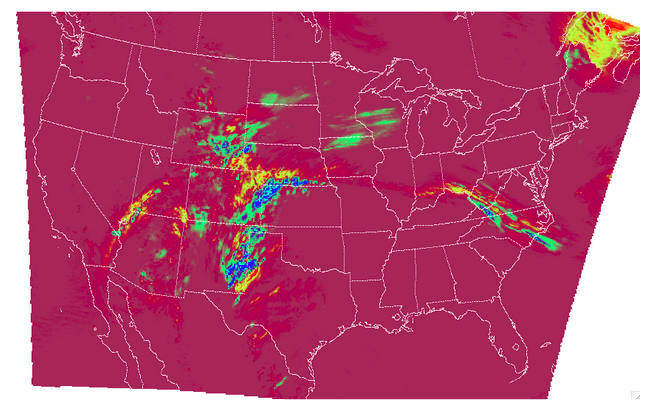
The resulting two files have a wealth of information and statistics. The netCDF output contains our visual confirmation that the forecast and observation input fields were interpreted correctly by MET, as well as the difference between the two fields which is provided below:

 For the CNT line type output we review the .stat file and find something similar to the following:

The columns that are available in the CNT line type are listed in the MET User’s Guide guidance for CNT line type {provide link here}. After the declaration of the line type (CNT), the familiar TOTAL or matched pairs column, we find a wealth of statistics including the forecast and observation means, the forecast and observation standard deviations, ME, MSE, along with all of the other statistics discussed in this section, all with their appropriate lower and upper confidence intervals and the bootstrap confidence intervals. Note that because the bootstrap library’s n_rep variable was kept at its default value of 0, bootstrap methods were not used and appear as NA in the stat file. You’ll also note that the ranking statistics (SP_CORR and KT_CORR) are listed as NA because we did not set rank_corr_flag to TRUE in the Grid-Stat configuration file. This was done intentionally; in order to calculate ranking statistics MET needs to assign each and every matched pair a rank and then perform the calculations. With a large dataset with numerous matched pairs this can significantly increase runtime and be computationally intensive. Given our example had over 1.5 million matched pairs, these statistics are best left to a smaller domain. Let’s create that smaller domain in a METplus wrappers example!

METplus Wrapper Example of Continuous Forecast Verification

To achieve the same success as the previous example but utilizing METplus wrappers instead of MET, very few adjustments would need to be made. Because METplus wrappers have the helpful feature of chaining multiple tools together, we’ll start off by listing all of the tools we want to use. Recall that for this example, we want to include a smaller verification area to enable the rank correlation statistics as well. This results in the following process list:

The second listing of GridStat uses the instance feature to allow a second run of Grid-Stat with different settings. Now we need to set the _VAR1 settings appropriately:

We’ve utilized a different setting, FCST_PCP_COMBINE_OUTPUT_NAME, to control what forecast variable name is verified. This way if a different forecast variable were to be used in a later run (assuming it had the same level dimensions as the precipitation), the forecast variable name would only need to be changed in one place instead of multiple. We also utilize METplus wrappers' ability to set an index based on a time, behaving similarly to the “@” usage in the MET example. Now we need to create all of the settings for PCPCombine:

From these settings, we see that all of the arguments from the command line for PCP-Combine are present: we will use the “add” method to loop over six netCDF files, each containing a variable field name of P01M_NONE and accumulation times of one hour. The output variable should be named APCP_06 and will be stored in the location as directed by FCST_PCP_COMBINE_OUTPUT_DIR and FCST_PCP_COMBINE_OUTPUT_TEMPLATE (not shown above).

Because the loop/timing information is controlled inside the configuration file for METplus wrappers (as opposed to MET’s non-looping option), that information must also be set accordingly, paying close attention that both instances of GridStat and PCPCombine will behave as expected:

Recall that we need to perform the verification on an alternate grid for one of the instances, and a small subset of the larger area in the other. So in the first instance configuration file area (anywhere outside of the [rank] instance configuration file area) we add

And set the [rank] instance up as follows:

For this instance of GridStat, we’ve set our own verification area using the grid definition option {link grid project here}, and utilized the OVERRIDES option {link to the OVERRIDES discussion here} to set the rank_corr_flag option, which is currently not a METplus wrapper option, to TRUE. Because both GridStat instances will create CNT output, the [rank] instance CNT output would normally overwrite the first GridStat instance. To avoid this, we create a new output template for the [rank] instance of GridStat to follow, preserving both files.

Finally, the desired line types and nc_pairs_flag settings need to be selected for output. This can be done outside of the [rank] instance, as any setting that is not overwritten by an instance further down the configuration file will be propagated to all applicable tools in the configuration file:

With a proper setting of the input and output directories, file templates, and a successful run of METplus, the same .stat output and netCDF file that were created in the MET example would be produced here, complete with CNT line type. However this example would result in two additional files: one .stat file that contains values for the rank correlation statistics and a netCDF file with the smaller area that was used to calculate them. The contents of that second .stat file would look something like the following:

We can see the smaller verification area resulted in only 1,600 matched pairs, which is much more reasonable for rank computations. SP_CORR was 0.41127 showing a positive correlation, while KT_CORR was 0.28929, a slightly weaker positive correlation. METplus goes the additional step and also shows that of the 1,600 ranks that were used to calculate KT_CORR, it found 1,043 forecast ranks that were tied and 537 observation ranks that were tied. Not something that would be easily computed without the help of METplus!