METplus Practical Session Guide (Version 5.0) | Binary Categorical Forecasts > METplus Examples of Binary Categorical Forecast Verification

The following two examples show a generalized method for calculating binary categorical statistics: one for a MET-only usage, and the same example but utilizing METplus wrappers. These examples are not meant to be completely reproducible by a user: no input data is provided, commands to run the various tools are not given, etc. Instead, they serve as a general guide of one possible setup among many that produce binary categorical statistics.

If you are interested in reproducible, step-by-step examples of running the various tools of METplus, you are strongly encouraged to review the METplus online tutorial that follows this statistical tutorial, where data is made available to reproduce the guided examples.

In order to better understand the delineation between METplus, MET, and METplus wrappers which are used frequently throughout this tutorial but are NOT interchangeable, the following definitions are provided for clarity:

• METplus is best visualized as an overarching framework with individual components. It encapsulates all of the repositories: MET, METplus wrappers, METdataio, METcalcpy, and METplotpy.
• MET serves as the core statistical component that ingests the provided fields and commands to compute user-requested statistics and diagnostics.
• METplus wrappers is a suite of Python wrappers that provide low-level automation of MET tools and plotting capability. While there are examples of calling METplus wrappers without any underlying MET usage, these are the exception rather than the rule.

MET Example of Binary Categorical Forecast Verification

This example demonstrates categorical forecast verification in MET.

For this example, let’s examine Grid-Stat. Assume we wanted to verify a binary temperature forecast of greater than 86 degrees Fahrenheit. Starting with the general Grid-Stat configuration file, the following would resemble the minimum necessary settings/changes for the fcst and obs dictionaries:

We can see that the forecast field name in the forecast input file is named TMP, and is set accordingly in the fcst dictionary. Similarly, the Z0 level is used to grab the lowest (0th) vertical level the TMP variable appears on. Finally, cat_thresh, which controls the categorical threshold that the contingency table will be created with, is set to greater than 86.0. This assumes that the temperature units in the file are in Fahrenheit. The obs dictionary is simply copying the settings from the fcst dictionary, which is a method that can be used if both the forecast and observation input files share the same variable structure (e.g. both inputs use the TMP variable name, in Fahrenheit, with the lowest vertical level being the desired verification level).

Now all that’s necessary would be to adjust the output_flag dictionary settings to have Grid-Stat print out the desired line types:

In this example, we have told MET to output the CTC and CTS line types, which will contain all of the scalar statistics that were discussed in this section. Running this set up would produce one .stat file with the two line types that were selected, CTC and CTS. The CTC line would look something like:

While the stat file full header column contents are discussed in the User’s Guide, the CTC line types are the final 6 columns of the line, beginning after the “CTC” column. The first value is MET’s TOTAL column which is the “total number of matched pairs”. You might better recognize this value as n, the summation of every cell in the contingency table. In fact, the following four columns of the CTC line type are synonymous with the contingency table terms, which have their corresponding MET terms provided in this table for your convenience:

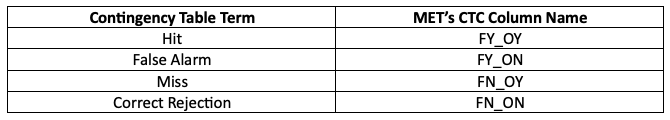
Further descriptions of each of the CTC columns can be found in the MET User’s Guide. Note that the final column of the CTC line type, EC_VALUE, is only relevant to users verifying probabilistic data with the HSS_EC skill score.

The CTS line type is also present in the .stat file and is the second row. It has many more columns than the CTC line, where all of the scalar statistics and skill scores discussed previously are located. Focusing on the first few columns of the example output, you would find:

These columns can be understood by reviewing the MET User’s Guide guidance for CTS line type. After the familiar TOTAL or n column, we find statistics such as Base Rate, forecast mean, Accuracy, plus many more, all with their appropriate lower and upper confidence intervals and the bootstrap confidence intervals. Note that because the bootstrap library’s n_rep variable was kept at its default value of 0, bootstrap methods were not used and appear as NA in the stat file. While all of these statistics could be obtained from the CTC line type values with additional post-processing, the simplicity of having all of them already calculated and ready for additional group statistics or to advise forecast adjustments is one of the many advantages of using the METplus system.

METplus Wrapper Example of Binary Categorical Forecast Verification

To achieve the same outcome as the previous example but utilizing METplus wrappers instead of MET, very few changes would need to be made. Starting with the standard GridStat configuration file, we would need to set the _VAR1 settings appropriately:

Note how the BOTH option is utilized here (as opposed to individual FCST_ and OBS_ settings) since the forecast and observation datasets utilize the same name and level information. Because the loop/timing information is controlled inside the configuration file for METplus wrappers (as opposed to MET’s non-looping option), that information must also be set accordingly:

Finally, the desired line types need to be selected for output. In the wrappers, that looks like this:

After a successful run of METplus, the same .stat output file that was created in the MET example would be produced here, complete with CTC and CTS line type rows.