METplus Practical Session Guide (Version 5.0)
METplus Practical Session Guide (Version 5.0)
Welcome to the METplus Practical Session Guide
The METplus v5.0.0 practical consists of 11 sessions. The first six sessions contain instructions for running individual MET tools directly on the command line, followed by instructions for running the same tools as part of a METplus use case. The remaining sessions dive into special applications of METplus and the Analysis tools available in the METplus suite.
Please follow the link to the appropriate session:
- Session 1
METplus Setup/Grid-to-Grid - Session 2
Grid-to-Obs - Session 3
Analysis Tools - Session 4
Ensemble and PQPF - Session 5
MODE and MTD - Session 6
Track and Intensity - Session 7
Feature Relative - Session 8
METplus Analysis Tools - Session 9
Python Embedding - Session 10
Subseasonal To Seasonal (S2S) - Session 11
METplus Cloud
Basic Verification Statistics Review
Basic Verification Statistics Review
Introduction
This session is meant as a brief introduction (or review) of basic statistical verification methods applied for various classifications of meteorological variables, and to guide new users toward their usage within the METplus system. It is by no means a comprehensive review of all of the available statistical verification methods available in the atmospheric sciences, nor every single verification method available within the METplus system. More complete details on many of the techniques discussed here can be found in Wilks’ “Statistical Methods In The Atmospheric Sciences” (2019), Jolliffe and Stephenson’s “Forecast Verification; A Practitioner's Guide in Atmospheric Science” (2012) and the forecast verification web page hosted by Australia’s Bureau of Meteorology. Upon completion of this session you will have a better understanding of five of the common classification groupings for meteorological verification and have access to generalized METplus examples of creating statistics from those categories.
Attributes of Forecast Quality
Attributes of Forecast Quality
Attributes of Forecast Quality
Forecast quality attributes are the basic characteristics of forecast quality that are of importance to a user and can be assessed through verification. Different forecast evaluation approaches will measure different attributes of the quality of the forecasts. Some verification statistics can be decomposed into several attributes, providing more nuance to the quality information. It can be commonplace in operational and research settings to find and settle on one or two of these complex statistics that can provide meaningful guidance for adjustments to the model being evaluated. For example, if a given verification statistic shows that a model has a high bias and low reliability, that can seem to provide a researcher with all they need to know to make the next iteration of the model perform better, having no need for any other statistical input. However, this is an example of the law of the instrument: “If the only tool you have is a hammer, you tend to see every problem as a nail”. More complete, meaningful verification requires examining forecast performance from multiple perspectives and applying a variety of statistical approaches that measure a variety of verification attributes.
In most cases, one or two forecast verification attributes will not provide enough information to understand the quality of a forecast. In the previous example where one verification statistic showed a model had high bias and low reliability, it could have been a situation where a second verification measure would have shown that the accuracy and resolution of the model were good, and making the adjustments to the next model iteration to correct bias and reliability would degrade accuracy and resolution. To fully grasp how well a particular forecast is performing, it is important to select the right combination of statistics that give you the “full picture” of the forecasts’ performance, which may consist of a more complete set of attributes, measuring the overall quality of your set of forecasts.
The following forecast attribute list is taken from Wilks (2019) and summarized for your convenience. Note how statistics showing one of these attributes on their own will not tell you exactly how “good” a forecast is, but combined with statistics showcasing other attributes you can have a better understanding of the utility of the forecast.
- Accuracy – The level of difference (or agreement) between the individual values of a forecast dataset and the individual values of the observation dataset. This should not be confused with the informal usage of “accurate”, which is often used by the general population to describe a forecast that has high quality.
- Skill – The accuracy of a forecast relative to a reference forecast. The reference forecast can be a single or group of forecasts that are compared against, with common choices being climatological values, persistence forecasts (forecasts that do not change over time), and older numerical model versions.
- Bias – The similarity between the mean forecast and mean observation. Note that this differs slightly from the accuracy attribute, which measures the individual value’s similarity.
- Reliability – The agreement between conditional forecast values and the distribution of the observation values resulting from that condition. Another way to think of reliability is as a measure of all of the observational value distributions that could happen given a forecast value.
- Resolution – In a similar thought as reliability, resolution is the measure of the forecast’s ability to resolve different observational distributions given a change in the forecast value. Simply put, if value X is forecast, what level of difference is there in the resulting observation distributions than a forecast of value Y.
- Discrimination – A simpler definition could be considered the inverse of resolution: discrimination is the measure of a forecast’s distribution given a change in the observation value. For example, if a forecast is just as likely to predict a tornado regardless of the actual observation of a tornado occurring, that forecast would have a low discrimination ability for tornadoes.
- Sharpness – This property pertains only to the forecast with no consideration of its observational pair. If the forecast does not deviate from a consistent (e.g., climatological) distribution, and instead sticks close to a “climatological value”, it exhibits low sharpness. If the forecast has the ability to produce values different from climatology that change the distribution, then it demonstrates sharpness.
Binary Categorical Forecasts
Binary Categorical Forecasts
Binary Categorical Forecasts
The first group of verification types to consider is one of the more basic, but most often used. Binary categorical forecast verification seeks to answer the question “did the event happen”. Some variables (e.g., rain/no rain) are by definition binary categorical, but every type of meteorological variable can be evaluated in the context of a binary forecast (e.g., by applying a threshold): Will the temperature exceed 86 degrees Fahrenheit? Will wind speeds exceed 15 knots? These are just some examples where the observations fall into one of only two categories, yes or no, which are created by the two categories of the forecast (e.g. the temperature will exceed 86 degrees Fahrenheit, or it will stay at or below 86 degrees Fahrenheit).
Imagine a simplified scenario where the forecast calls for rain.
A hit occurs when a forecast predicts a rain event and the observation shows that the event occurred. In the scenario, a hit would be counted if rain was observed. A false alarm would be counted when the forecast predicted an event, but the event did not occur (i.e., in the scenario, this would mean no rain was observed). As you may have figured out, there are two other possible scenarios to cover for when the forecast says an event will not occur.
To describe these, imagine a second scenario where the forecast says there will be no rain.
Misses count the occasions when the forecast does not predict the event to occur, but it is observed. In this new scenario, a miss would be counted if rain was observed. Finally, correct rejections are those times that a forecast says the event will not occur, and observations show this to be true. Thus, in the rainfall scenario a correct rejection would be counted if no rain was forecasted and no rain was observed.
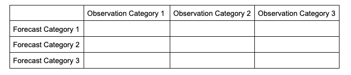
Because forecast verification is rarely performed on one event, a contingency table can be utilized to quickly convey the results of multiple events that all used the same binary event conditions. An example contingency table is shown here:
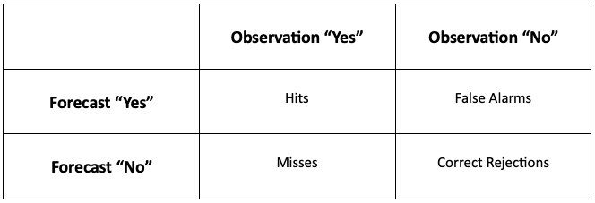
Each of the paired categorical forecasts and observations can be assigned to one of the four categories of the contingency table. The statistics that are used to describe the categorical forecasts’ scalar attributes (accuracy, bias, reliability, etc.) are computed using the total counts in these categories.
It is important not to forget the total number of occurrences and non-occurrences, n, that are contained in all four categories. If n is too small, it can be easy to arrive at a misleading conclusion. For example, if a forecaster claims 100% accuracy in their rain forecast and produces a contingency table where the forecast values were all hits but n=4, the conclusion is technically correct, but not very scientifically sound!
Verification Statistics for Binary Categorical Forecasts
Verification Statistics for Binary Categorical Forecasts
Verification Statistics for Binary Categorical Forecasts
Most meteorological forecasts would be described as non-probabilistic, meaning the forecast value given is provided with no additional information of certainty in that value. Another term for this type of forecast is deterministic and will be the focus of the verification statistics in this section. For more information on probabilistic forecasts and their corresponding statistics please refer to the probabilistic section. When verifying binary categorical forecasts, the only important factor is whether or not the event occurred: the assumed certainty in the forecast is 100%.
Numerous computationally-easy (and very popular) scalar statistics are within reach without too much manipulation of a contingency table’s counts.
Accuracy (Acc)
The scalar attribute of Accuracy is measured as a simple ratio between the forecasts that correctly predicted the event and the total number of occurrences and non-occurrences, n. In equation format,
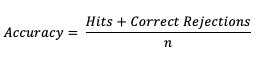
This measure (often called “Percent Correct”) is very easily computed and addresses how often a forecast is correctly predicting an event and non-event. As most verification resources will warn you, however, this measure should be used with caution, especially for an event that happens only rarely. The Finley tornado forecast study (1884) is an excellent example of the need for caution, with Finley reporting a 96.6% Accuracy for predicting a tornado due to the overwhelming count of correct negatives. Peers were quick to point out that a higher Accuracy (98.2%) could have been achieved with a persistence forecast of No Tornado! See how to use this statistic in METplus!
Probability of Detection (POD)
Probability of Detection (POD), also referred to as the Hit Rate, measures the frequency that the forecasts were correct given that the forecast predicts an occurrence. Rather than computing the ratio of the correct forecasts to the entire occurrence and non-occurrence count (i.e., as in Accuracy), POD only focuses on the times the forecast predicted an event would occur. Thus, this measure is categorized as a discrimination statistic. POD is computed as
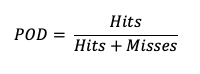
This measure is useful for rare events (tornadoes, 100-year floods, etc.) as it will penalize (i.e. go toward 0) the forecasts when there are too many missed forecasts. See how to use this statistic in METplus!
Probability of False Detection (POFD)
A countermeasure to POD is the probability of false detection (POFD). POFD (also called false alarm rate), measures the frequency of false alarm forecasts relative to the frequency that an event does not occur.
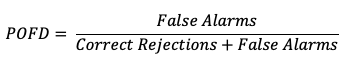
Together, POD and POFD measure forecasts’ ability to discriminate between occurrences and non-occurrences of the event of interest. See how to use this statistic in METplus!
Frequency bias (Bias)
Frequency bias (a measure of, you guessed it, bias!) compares the count of “yes” forecasts to the count of “yes” events observed.
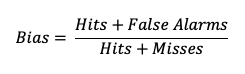
This ratio does not provide specific information about the performance of individual forecasts, but rather is a measure of over- or under-forecasting of the event. See how to use this statistic in METplus!
False Alarm Ratio (FAR)
The False Alarm Ratio (FAR) provides information about both the reliability and resolution attributes of forecasts. It computes the ratio of “yes” forecasts that did not occur to the total number of times a “yes” forecast was made (i.e., the proportion of “yes” forecasts that were incorrect).
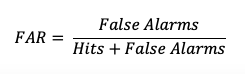
FAR also is the first statistic covered in this session that has a negative orientation: a FAR of 0 is desirable, while a FAR of 1 shows the worst possible ratio of “yes” forecasts that were not observed relative to total “yes” forecasts. See how to use this statistic in METplus!
Critical Success Index (CSI)
The Critical Success Index (CSI), also commonly known as the Threat Score, is a second measure of the overall accuracy of forecasts (e.g., like the Accuracy measure mentioned earlier). Accuracy pertains to the agreement of individual forecast-observation pairs, and CSI can be calculated as
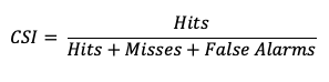
Note that by definition CSI can be described as the ratio between the times the forecast correctly called for an event and the total times the forecast called for an event or the event was observed. Thus, CSI ignores correct negatives, which differentiates it from percent correct. A CSI of 1 indicates a highly accurate forecast, while a value of 0 indicates no accuracy. See how to use this statistic in METplus!
Binary Categorical Skill Scores
Binary Categorical Skill Scores
Binary Categorical Skill Scores
Skill scores can be a more meaningful way of describing a forecast’s quality. By definition, skill scores compare the performance of the forecasts to some standard or “reference forecast” (e.g., climatology, persistence, perfect forecasts, random forecasts). They often combine aspects of the previously-listed scalar statistics and can serve as a starting point for creating your own skill score that is better suited to your forecasts’ properties. Skill scores create a summary view of the contingency table, which is in contrast to the scalar statistics’ focus on one attribute at a time.
Three of the most popular skill statistics for categorical variables are the Heidke Skill Score (HSS), the Hanssen-Kuipers Discriminant (HK), and the Gilbert Skill Score (GSS). These measures are described here.
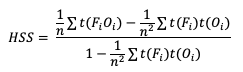
Heidke Skill Score (HSS)
The HSS measures the proportion correct relative to the expected proportion correct that would be achieved by a “reference” forecast, denoted by C2 in the equation. In this instance, the reference forecast denotes a forecast that is completely independent of the observation dataset. In practice, the reference forecast often is based on a random, climatology, or persistence forecast. By combining the probability of a correct “yes” forecast (i.e., a hit) with the probability of a correct “no” forecast (i.e. a correct rejection) the resulting equation is
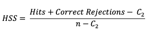
HSS can range from -1 to 1, with a perfect forecast receiving a score of 1. The equation presented above is a compact version which uses a sample climatology, C2 based on the counts in the contingency table. The C2 term expands to

This is a basic “traditional” version of HSS. METplus also calculates a modified HSS, that allows users to control how the C2 term is defined. This additional control allows users to apply an alternative standard of comparison, such as another forecast or a basic standard such as a persistence forecast or climatology. See how to use these skill scores in METplus!
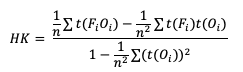
Hanssen-Kuipers Discriminant (HK)
HK is known by several names, including the Peirce Skill Score and the True Skill Statistic. This score is similar to HSS (ranges from -1 to 1, perfect forecast is 1, etc.). HK is formulated relative to a random forecast that is constrained to be unbiased. In general, the focus of the HK is on how well the forecast discriminates between observed “yes” events and observed “no” events. The equation for HK is
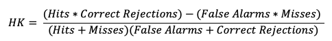
which is equivalent to “POD minus POFD”. Because of its dependence on POD, HK can be similarly affected by infrequent events and is suggested as a more useful skill score for frequent events. See how to use this skill score in METplus!
Gilbert Skill Score (GSS)
Finally, GSS measures the correspondence between forecasted and observed “yes” events. Sometimes called the Equitable Threat Score (ETS), GSS is a good option for those forecasted events where the observed “yes” event is rare. In particular, the number of correct negatives (which for a rare event would be large) are not considered in the GSS equation and thus do not influence the GSS values. The GSS is given as
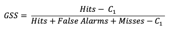
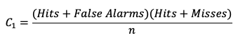
GSS ranges from -1 to 1, with a perfect forecast receiving a score of 1. Similar to HSS, a compact version of GSS is presented using the C1 term. This term expands to
METplus solutions for Binary Categorical Forecast Verification
METplus solutions for Binary Categorical Forecast Verification
METplus solutions for Binary Categorical Forecast Verification
Now that you know a bit more about dichotomous, deterministic forecasts and how to extract information on the scalar attributes through statistics, it’s time to show how you can access those same statistics in METplus!
In order to better understand the delineation between METplus, MET, and METplus wrappers which are used frequently throughout this tutorial but are NOT interchangeable, the following definitions are provided for clarity:
- METplus is best visualized as an overarching framework with individual components. It encapsulates all of the repositories: MET, METplus wrappers, METdataio, METcalcpy, and METplotpy.
- MET serves as the core statistical component that ingests the provided fields and commands to compute user-requested statistics and diagnostics.
- METplus wrappers is a suite of Python wrappers that provide low-level automation of MET tools and plotting capability. While there are examples of calling METplus wrappers without any underlying MET usage, these are the exception rather than the rule.
MET solutions
The MET User’s Guide provides an Appendix that dives into all of the statistical measure that MET calculates. METplus groups statistics together by application and type and makes them available to METplus users via several line types. For example, many of the statistics that were discussed above can be found in the Contingency Table Statistics (CTS) line type, which logically groups together statistics based directly on contingency table counts. In fact, MET allows users to directly access the contingency table counts through the aptly named Contingency Table Counts (CTC) line type.
The line types that are output by MET depend on your selection of the appropriate line type using the output_flag dictionary. Note that certain line types may or may not be available in every tool: for example, both Point-Stat and Grid-Stat produce CTS line types, which allow users to access the various contingency table statistics for both point-based observations and gridded observations. In contrast, Ensemble-Stat is the only tool that can generate a Ranked Probability Score (RPS) line type, which provides statistics relevant to the analysis of ensemble forecasts. If you don’t see your desired statistic in the line type or tool you’d expect it to be in, be sure to check the Appendix to see if the statistic is available in MET and which line type it’s currently grouped with.
As for the categorical statistics that were just discussed, here’s a link to the User’s Guide Appendix entry that discusses their use in MET:
Remember that for categorical statistics, including those that are associated with probabilistic datasets, you will need to provide an appropriate threshold that divides the observations and forecasts into two mutually exclusive categories. For more information on the available thresholding options, please review this section of the MET User’s Guide.
METplus Wrapper Solutions
The same statistics that are available in MET are also available with the METplus wrappers. To better understand how MET configuration options for the selection of statistics translate to METplus wrapper configuration options, you can utilize the Statistics and Diagnostics Section of the METplus wrappers User’s Guide, which lists all of the available statistics through the wrappers, including which tools can output particular statistics. To access the line types through the tool, select your desired tool and use this page to view a list of all available commands for that tool. Once you do, you’ll see that the tool will include several options that contain _OUTPUT_FLAG_. These options will exhibit the same behavior and accept the same settings as the line types in MET’s output_flag dictionary, so be sure to review the available settings to get the line type output you want.
METplus Examples of Binary Categorical Forecast Verification
METplus Examples of Binary Categorical Forecast Verification
The following two examples show a generalized method for calculating binary categorical statistics: one for a MET-only usage, and the same example but utilizing METplus wrappers. These examples are not meant to be completely reproducible by a user: no input data is provided, commands to run the various tools are not given, etc. Instead, they serve as a general guide of one possible setup among many that produce binary categorical statistics.
If you are interested in reproducible, step-by-step examples of running the various tools of METplus, you are strongly encouraged to review the METplus online tutorial that follows this statistical tutorial, where data is made available to reproduce the guided examples.
In order to better understand the delineation between METplus, MET, and METplus wrappers which are used frequently throughout this tutorial but are NOT interchangeable, the following definitions are provided for clarity:
- METplus is best visualized as an overarching framework with individual components. It encapsulates all of the repositories: MET, METplus wrappers, METdataio, METcalcpy, and METplotpy.
- MET serves as the core statistical component that ingests the provided fields and commands to compute user-requested statistics and diagnostics.
- METplus wrappers is a suite of Python wrappers that provide low-level automation of MET tools and plotting capability. While there are examples of calling METplus wrappers without any underlying MET usage, these are the exception rather than the rule.
MET Example of Binary Categorical Forecast Verification
This example demonstrates categorical forecast verification in MET.
For this example, let’s examine Grid-Stat. Assume we wanted to verify a binary temperature forecast of greater than 86 degrees Fahrenheit. Starting with the general Grid-Stat configuration file, the following would resemble the minimum necessary settings/changes for the fcst and obs dictionaries:
field = [
{
name = "TMP";
level = [ "Z0" ];
cat_thresh = [ >86.0 ];
}
];
}
obs = fcst;
We can see that the forecast field name in the forecast input file is named TMP, and is set accordingly in the fcst dictionary. Similarly, the Z0 level is used to grab the lowest (0th) vertical level the TMP variable appears on. Finally, cat_thresh, which controls the categorical threshold that the contingency table will be created with, is set to greater than 86.0. This assumes that the temperature units in the file are in Fahrenheit. The obs dictionary is simply copying the settings from the fcst dictionary, which is a method that can be used if both the forecast and observation input files share the same variable structure (e.g. both inputs use the TMP variable name, in Fahrenheit, with the lowest vertical level being the desired verification level).
Now all that’s necessary would be to adjust the output_flag dictionary settings to have Grid-Stat print out the desired line types:
fho = NONE;
ctc = STAT;
cts = STAT;
mctc = NONE;
mcts = NONE;
cnt = NONE;
…
In this example, we have told MET to output the CTC and CTS line types, which will contain all of the scalar statistics that were discussed in this section. Running this set up would produce one .stat file with the two line types that were selected, CTC and CTS. The CTC line would look something like:
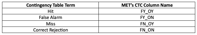
While the stat file full header column contents are discussed in the User’s Guide, the CTC line types are the final 6 columns of the line, beginning after the “CTC” column. The first value is MET’s TOTAL column which is the “total number of matched pairs”. You might better recognize this value as n, the summation of every cell in the contingency table. In fact, the following four columns of the CTC line type are synonymous with the contingency table terms, which have their corresponding MET terms provided in this table for your convenience:
Further descriptions of each of the CTC columns can be found in the MET User’s Guide. Note that the final column of the CTC line type, EC_VALUE, is only relevant to users verifying probabilistic data with the HSS_EC skill score.
The CTS line type is also present in the .stat file and is the second row. It has many more columns than the CTC line, where all of the scalar statistics and skill scores discussed previously are located. Focusing on the first few columns of the example output, you would find:
These columns can be understood by reviewing the MET User’s Guide guidance for CTS line type. After the familiar TOTAL or n column, we find statistics such as Base Rate, forecast mean, Accuracy, plus many more, all with their appropriate lower and upper confidence intervals and the bootstrap confidence intervals. Note that because the bootstrap library’s n_rep variable was kept at its default value of 0, bootstrap methods were not used and appear as NA in the stat file. While all of these statistics could be obtained from the CTC line type values with additional post-processing, the simplicity of having all of them already calculated and ready for additional group statistics or to advise forecast adjustments is one of the many advantages of using the METplus system.
METplus Wrapper Example of Binary Categorical Forecast Verification
To achieve the same outcome as the previous example but utilizing METplus wrappers instead of MET, very few changes would need to be made. Starting with the standard GridStat configuration file, we would need to set the _VAR1 settings appropriately:
BOTH_VAR1_LEVELS = Z0
BOTH_VAR1_THRESH = gt86.0
Note how the BOTH option is utilized here (as opposed to individual FCST_ and OBS_ settings) since the forecast and observation datasets utilize the same name and level information. Because the loop/timing information is controlled inside the configuration file for METplus wrappers (as opposed to MET’s non-looping option), that information must also be set accordingly:
INIT_TIME_FMT = %Y%m%d%H
INIT_BEG=2023080700
INIT_END=2023080700
INIT_INCREMENT = 12H
LEAD_SEQ = 12
Finally, the desired line types need to be selected for output. In the wrappers, that looks like this:
GRID_STAT_OUTPUT_FLAG_CTS = STAT
After a successful run of METplus, the same .stat output file that was created in the MET example would be produced here, complete with CTC and CTS line type rows.
Multicategorical Forecasts
Multicategorical Forecasts
Multicategorical Forecasts
In practical applications of forecast verification, it’s often of interest to look at more than two categories and cannot be reduced to a binary, “did the event happen or not, and was the event forecasted or not”. Restricting forecast and observation datasets to binary options leads to the loss of important information about how the forecast performed (e.g., when multiple categories are combined into just two categories). For example, if the forecast called for rain but snow was observed instead, it can be useful to analyze how “good” the forecast was at delineating between rain, snow, and any other precipitation type. Luckily, the transformation of statistics from supporting binary categorical forecasts to the second group of forecasts, multi-category, is fairly straightforward.
Verification Statistics for Multicategorical Forecasts
Verification Statistics for Multicategorical Forecasts
Verification Statistics for Multicategorical Forecasts
In order to make sense of how the statistics are modified when evaluating multiple categories, it will help to look at how the contingency table changes. The generalized contingency table for a three category table will look like the following:
A similar table could be constructed for comparisons of four, five, six, and so on, categories. Some statistical calculations are more easily computed when forecasts and observations are restricted to two options (as was the case in binary categorical forecasts), so one less common approach for a multi-category contingency table is to process the full table into multiple instances of 2x2 grids, focusing on one forecast category at a time. This way, each forecasted event or category can have scalar attributes calculated, as well as skill scores that reflect the entire forecast’s quality across the multiple categories. This is not a valid approach for calculating, among others, Heidke Skill Score and Gilbert Skill Score, but is considered here for a well-rounded approach to multicategorical verification.
To demonstrate how scalar attributes are calculated for a multicategory forecast, imagine a scenario where the forecast can call for three separate precipitation types: rain, snow, and ice pellets. For this scenario, forecasts and observations of no precipitation are ignored (i.e., this evaluation is conditioned on some type of precipitation both occurring and being forecasted).
The contingency table would look like the following:
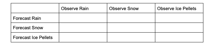
To extract the scalar attributes for rain, the simplified, 2x2 contingency table would look like this:
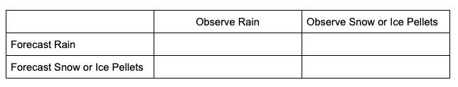
The same simplification can be done for snow and ice pellets. As this new 2x2 contingency table demonstrates, by reducing the multicategorical options to the binary choices of each forecasted event (e.g., did the forecast predict rain rather than snow or ice pellets, did the forecast predict snow rather than rain or ice pellets, did the forecast predict ice pellets rather than rain or snow) and evaluating the corresponding observations, scalar statistics such as POD, Bias, etc. can be calculated in the same method as the binary categorical forecasts.
One of the unique scalar statistics that does not need a contingency table simplification is Accuracy (Acc). This is due to its definition, which, when presented in its general format, becomes:
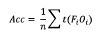
Note that t(FiOi) is the number of forecasts in category i of the multicategory contingency table that had an observation of Oi and n is the total number of occurrences and non-occurrences.
With this general format of Accuracy, essentially we seek to answer the question “how capable was the forecast at selecting the exact category?” To demonstrate how this would look in a 3x3 contingency table, let’s return to the previous scenario of a three precipitation type forecast. A perfect Accuracy forecast would have nonzero values only in the “Forecast Rain, Observation Rain”, “Forecast Snow, Observation Snow”, and “Forecast Ice Pellets, Observation Ice Pellets” cells, with the remaining cells being zero. The same top-left corner to lower-right corner of nonzero cells pattern would exist in the simplified 2x2 contingency table. Because no information about the forecast’s Accuracy is lost for the full count of forecast categories, Accuracy is the only scalar statistic that METplus will calculate from the full multicategory contingency table. See how to use this statistic in METplus!
Multicategorical Skill Scores
Multicategorical Skill Scores
Multicategorical Skill Scores
While some statistics for multicategorical forecasts require simplifying the contingency table to two-categories, and therefore only show the forecast’s quality in respect to the individual category, certain skill scores are designed to evaluate forecasts with multiple categories, allowing the skill score to reflect the quality of the entire forecast spectrum.
Heidke Skill Score (HSS)
HSS has a general form to accommodate multicategory forecasts. While more computationally intense than the two-category equation provided, the multi-category formulation is also based on comparison of the percent correct in the forecast relative to the proportion correct that would be achieved by a “random” forecast. The relative comparison is often with sources other than a “random” forecast, including older versions of a model and climatology. This general form is
Note that t(FiOi) is the number of forecasts in category i of the multicategory contingency table that had an observation of Oi, t(Fi) is the total number of forecasts in category i, and n is the total number of occurrences and non-occurrences.
Hanssen-Kuipers Discriminant (HK)
Similarly, HK is generalized to
Gerrity Skill Score
The Gerrity Skill Score is designed specifically for multicategory forecasts. While it is not as easily calculated as HSS and HK, it is useful for demonstrating the ability of the forecasts to delineate the correct event category when compared to random chance. The Gerrity Skill Score properly penalizes a forecast that has more than two options for an event, something not captured in the generalized forms of HSS or HK. This is achieved through the use of weights, sj,j, which correspond to correct forecasts, and sj,i, which represent weights for incorrect forecasts. These weights are given as
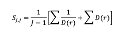
and
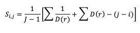
where D(r) is the likelihood ratio using dummy summation index r, calculated using
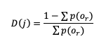
where p(or) is the probability of a sample climatology.
Finally, the Gerrity Skill Score is computed through summing the product of the scoring weights and their corresponding joint probability distribution. That distribution is found by taking each count of the contingency table cell and dividing it by the total number of occurrences and non-occurrences across all cells, n. See how to use these statistics in METplus!
METplus solutions for Multicategorical Forecast Verification
METplus solutions for Multicategorical Forecast Verification
METplus solutions for Multicategorical Forecast Verification
One important note regarding how to define multicategorical thresholds within the MET and METplus wrapper configuration files should be discussed. METplus requires that when multiple thresholds are listed using the cat_thresh variable to calculate any multicategorical line types, the thresholds must be monotonically increasing and use the same inequality type. This is done in order to ensure that the thresholds create unique and discrete bins of values, rather than overlapping thresholds that do not provide any sound statistical value. In practice, this means that the following two examples would result in a METplus error:
Example 1.
Example 2.
In example 1, the thresholds decrease with each entry which violates the requirement of monotonically increasing. With a simple reordering of the thresholds, example 1 can use the same thresholds and run with success:
In example 2, the final threshold uses a different inequality than the other two thresholds which violates the requirement that all multicategorical thresholds use the same inequality type. This rewrite of example 2 will provide the same information desired from the original thresholds, but will now successfully run in METplus:
This time, the rewrite changed the final inequality to match the first two while also keeping the final bin of values that METplus will calculate, >=15.5, consistent with the desired information. More information on how MET creates the value bins from multicategory thresholds is provided in the MET example of Multicategorical Forecast Verification.
Now that you know a bit more about verification measures for multicategorical, deterministic forecasts, it’s time to show how you can access those same statistics in METplus!
In order to better understand the delineation between METplus, MET, and METplus wrappers which are used frequently throughout this tutorial but are NOT interchangeable, the following definitions are provided for clarity:
- METplus is best visualized as an overarching framework with individual components. It encapsulates all of the repositories: MET, METplus wrappers, METdataio, METcalcpy, and METplotpy.
- MET serves as the core statistical component that ingests the provided fields and commands to compute user-requested statistics and diagnostics.
- METplus wrappers is a suite of Python wrappers that provide low-level automation of MET tools and plotting capability. While there are examples of calling METplus wrappers without any underlying MET usage, these are the exception rather than the rule
MET solutions
The MET User’s Guide provides an Appendix that dives into statistical measures that it calculates, as well as the line type it is a part of. Statistics are grouped together by application and type and are available to METplus users in line types. To delineate between the calculation method for binary categorical and multicategorical forecast skill scores, METplus has two pairs of separate, but similar line types. As discussed in detail in the Binary Categorical forecasts section, the Contingency Table Statistics (CTS) line type and Contingency Table Counts (CTC) line type are for users who want single category forecast statistics. It’s important to note that the CTS line type must also be utilized by users who want scalar statistics from multicategorical forecasts, except for Accuracy. To accomplish this, simply follow the guidance listed in the Verification Statistics section for Multicategorical Forecasts. The complements to CTS and CTC in the multicategory group are the aptly named Multicategory Contingency Table Statistics (MCTS) line type and Multicategory Contingency Table Counts (MCTC) line type. Similar to the CTC, MCTC allows direct access to each of the counts from the contingency table of multicategorical forecasts. MCTS contains all of the skill scores that were discussed in the Multicategorical Verification statistics section, as well as the scalar statistic Accuracy, which are linked to their appendix description here for your convenience (except for Gerrity, which does not appear in the appendix):
METplus Wrapper Solutions
The same statistics that are available in MET are also available with the METplus wrappers. To better understand how MET configuration options for statistics translate to METplus wrapper configuration options, you can utilize the Statistics and Diagnostics Section of the METplus wrappers User’s Guide, which lists all of the statistics available through the wrappers, including which tools can output which statistics. To access the line type through the tool, find your desired tool in the list of available commands for that tool. Once you do, you’ll see the tool will have several options that contain _OUTPUT_FLAG_, which will exhibit the same behavior and accept the same settings as the line types in MET’s output_flag dictionary, so be sure to review the available settings to get the line type output you want.
METplus Examples of Multicategorical Forecast Verification
METplus Examples of Multicategorical Forecast Verification
The following two examples show a generalized method for calculating multicategorical statistics: one for a MET-only usage, and the same example but utilizing METplus wrappers. These examples are not meant to be completely reproducible by a user: no input data is provided, commands to run the various tools are not given, etc. Instead, they serve as a general guide of one possible setup among many that produce multicategorical statistics.
If you are interested in reproducible, step-by-step examples of running the various tools of METplus, you are strongly encouraged to review the METplus online tutorial that follows this statistical tutorial, where data is made available to reproduce the guided examples.
In order to better understand the delineation between METplus, MET, and METplus wrappers which are used frequently throughout this tutorial but are NOT interchangeable, the following definitions are provided for clarity:
- METplus is best visualized as an overarching framework with individual components. It encapsulates all of the repositories: MET, METplus wrappers, METdataio, METcalcpy, and METplotpy.
- MET serves as the core statistical component that ingests the provided fields and commands to compute user-requested statistics and diagnostics.
- METplus wrappers is a suite of Python wrappers that provide low-level automation of MET tools and plotting capability. While there are examples of calling METplus wrappers without any underlying MET usage, these are the exception rather than the rule.
MET Example of Multicategorical Forecast Verification
Here is an example that demonstrates multicategorical forecast verification in MET.
For this example, let’s use Point-Stat. Assume we wanted to verify a multicategory forecast of wind speeds over the ocean. Specifically of interest are speed thresholds of near gale force (13.9 m/s), gale force (17.2 m/s), tropical storm (24.5 m/s), and hurricane (32.7 m/s). Starting with the general Point-Stat configuration file, the following would resemble minimum necessary settings/changes for the fcst and obs dictionaries:
field = [
{
name = "WIND";
level = [ "Z10" ];
cat_thresh = [ >=13.9, >=17.2, >=24.5, >=32.7 ];
}
];
}
obs = fcst;
In this example, the forecast field name in the forecast input file is named WIND, and is set accordingly in the fcst dictionary. Wind speed is one of the unique variables in METplus that can be calculated from the u and v components of a grib1 or grib2 file if wind speed is not present in the file. Assuming the input file is in a grib1 or grib2 format, MET will first check if a variable field WIND is present; if it is, MET will use the values in that field for analysis. If not, MET will check for the u-component (UGRD) and v-component (VGRD) fields and if found, compute the wind speed field for analysis. A level of Z10 is used to grab the vertical level of 10 that WIND appears on, which for this input file corresponds to the 10 meter level. Finally, cat_thresh, which controls the categorical threshold used to create the multicategory contingency table, is set to four separate thresholds, with each value corresponding to one of the wind speed thresholds of interest. The example’s chosen thresholds assume that the wind speed units in the file are in meters per second. All of the additional fcst field entries from the general Point-Stat configuration file were removed. Note how MET uses four thresholds to creates five unique, discrete bins of wind speeds with a contingency table that would look like the following:
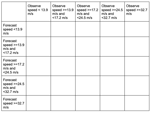
The table includes a “hidden” bin containing wind speeds less than 13.9 m/s that is not explicitly listed by a threshold in the MET settings, but rather implied: each of these bins is mutually exclusive and together they entail the complete real number line. This is why it is important to remember the “monotonically increasing and same inequality type” requirement when setting multicategorical forecast thresholds in METplus. For more discussion on this, review the METplus Solutions for Multicategorical Forecast Verification section.
The obs dictionary is simply copying the settings from the fcst dictionary, which is a method that can be used if both the forecast and observation input files share the same variable structure and file type (e.g. both inputs use the WIND variable name, in m/s, with the Z10 level corresponding to the 10 meter level).
Now all that’s necessary is to adjust the output_flag dictionary settings to have Point-Stat print out the desired line types:
fho = NONE;
ctc = NONE;
cts = NONE;
mctc = STAT;
mcts = STAT;
cnt = NONE;
…
In this example, we have told MET to output the MCTC and MCTS line types, which will produce one .stat file with the two line types that were selected. The MCTC line would look something like:
While the stat file full header column contents are discussed in the User’s Guide, the MCTC line types are the final columns of the line beginning after the “MCTC” column. The first value is MET’s TOTAL column which is the “total number of matched pairs”. You might better recognize this value as n, the summation of every cell in the contingency table. The following value is the number of dimensions or bins of the contingency table. As discussed above, providing four categorical thresholds creates a 5x5 contingency table. That means that we expect, and receive, 25 cells of data that make up the contingency table. They are listed starting with the lowest forecast and observation threshold pair, with increasing observation thresholds starting first. For the contingency table provided in this example, it would look like the following:
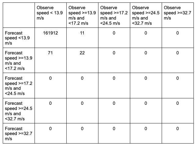
Note that the final column of the MCTC line type, EC_VALUE, is only relevant to users verifying probabilistic data with the HSS_EC skill score.
The MCTS line type is also present in the .stat file as the second row. In this example, the contents would be:
Compared to the statistics available in the CTC line type for dichotomous categorical forecasts, fewer verification statistics can be applied to a multicategorical contingency table, since most of the contingency table verification statistics require a simplified 2x2 contingency table. The columns that are available in the MCTS line type are listed in the MET User’s Guide guidance for the MCTS line type. After the declaration of the line type (MCTS), the familiar TOTAL or n column, and the number of bins created from the thresholds provided, we find Accuracy, HK, HSS, the Gerrity Skill Score, and HSS_EC, all with their appropriate lower and upper confidence intervals and the bootstrap confidence intervals. Accuracy has an additional two columns that give the normal confidence limits in addition to the bootstrap confidence limits. Note that because the bootstrap library’s n_rep variable was kept at its default value of 0, bootstrap methods were not used and appear as NA in the stat file. While all of these statistics could be obtained from the MCTC line type values with additional post-processing, the simplicity of having all of them already calculated and ready for additional group statistics or to advise forecast adjustments is one of the many advantages of using the METplus system.
METplus Wrapper Example of Multicategorical Forecast Verification
To achieve the same success as the previous example but utilizing METplus wrappers instead of MET, very few adjustments would need to be made. Starting with the standard PointStat configuration file, we would need to set the _VAR1 settings appropriately:
BOTH_VAR1_LEVELS = Z10
BOTH_VAR1_THRESH = ge13.9, ge17.2, ge24.5, ge32.7
Note how the BOTH option is utilized here (as opposed to individual FCST_ and OBS_ settings) since the forecast and observation datasets utilize the same name and level information. Because the loop/timing information is controlled inside the configuration file for METplus wrappers (as opposed to MET’s non-looping option), that information must also be set accordingly:
INIT_TIME_FMT = %Y%m%d%H
INIT_BEG=2023080700
INIT_END=2023080700
INIT_INCREMENT = 12H
LEAD_SEQ = 12
Finally, the desired line types need to be selected for output. In the wrappers, that looks like this:
GRID_STAT_OUTPUT_FLAG_MCTS = STAT
With a proper setting of the input and output directories, file templates, and a successful run of METplus, the same .stat output file that was created in the MET example would be produced here, complete with MCTC and MCTS line type rows.
Continuous Forecasts
Continuous Forecasts
Continuous Forecasts
When considering a forecast, one of the essential aspects is the actual value predicted by the forecast. For example, a forecast for 2 meter maximum air temperature of 75 degrees Fahrenheit is explicitly calling for one value to occur as the highest recorded temperature value for the entire day for that single point in space. If the maximum observed 2 meter air temperature was 77 degrees Fahrenheit for that point instead, then the forecast was incorrect: some might consider this the end of the story, another “blown” forecast. However, if the entire spectrum of 2-meter air temperature forecasts that could have been forecasted is considered, however, we can ask the question “how good or bad was that forecast, really”? After all, wasn’t the forecast only 2 degrees Fahrenheit off from what was observed? Continuous forecast verification is a category of verification that considers the entire real value spectrum that a forecast variable can take on, rather than individual discrete points or categories as is the case with dichotomous and multicategorical verification.
Verification Statistics for Continuous Forecasts
Verification Statistics for Continuous Forecasts
Verification Statistics for Continuous Forecasts
The nature of continuous forecast verification is a direct comparison of the forecast and observed values and measurement of the relationship of those two values over the real number range. We can easily infer that the scalar statistics and skill scores used for these kinds of forecasts will be different from those used for binary and multi-categorical forecasts. In fact many of the statistics that are used as “introductory statistics” are derived for continuous verification along the real number range, as continuous verification is a natural way we look at forecasts (i.e., how close or far the forecast and observed values are from each other).
Mean Errors
The simplest continuous measure is the mean error (ME), which is the average difference between two groups of data. So when you see “error” it is simply a measure of a difference. ME is calculated as
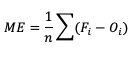
ME can range over the real numbers and has the obvious advantage of providing immediate insight into how far away, on average, the forecast values are from their corresponding observations. It is extremely easy to calculate, with a perfect forecast (i.e., a forecast that exactly corresponds to the observations) characterized by an ME of 0. ME serves as an important measurement of arithmetic bias. As a measure of bias, ME does not include a method for compensating for the magnitude of the differences between the forecast-observation pairs, and a forecast that has compensating errors could receive a mean error of 0. Essentially, ME provides an indication of whether a forecast has errors that - on average - are centered on zero; or if it is overforecasting or underforecasting on average. Consider the following scenario for wind speed forecasts at the same location for four different times:
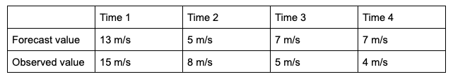
You’ll find the ME computed with these data equals 0, even though the difference between forecast and observation values for all of the times are non-zero. That’s because those errors that are positive (the forecast was greater than the observed value) are exactly negated by those errors that are negative (the forecast was less than the observed value). As noted earlier, ME is a good measure of bias; however, it is not a measure of accuracy.
This ability to effectively “hide” errors calls for a more robust error calculation to understand the forecasts’ accuracy. To that end, a few additional choices for measuring error are available.
Mean absolute error (MAE), while similar to ME, examines the absolute values of the errors, which are summed and averaged, providing a measure of accuracy as opposed to bias. Examining the absolute values of the errors restricts MAE’s range from zero to positive infinity, with a perfect score of zero:
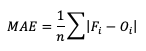
MAE also differs from ME in that it measures forecast accuracy, while ME measures bias. MAE provides a summary of the average magnitudes of the errors, but does not provide information about the direction (positive or negative) of the error magnitude.
Mean Squared Error (MSE) is another statistic focused on the characteristics of the forecast errors that measures forecast accuracy. In particular, MSE summarizes the squared differences between the forecast and observed values:
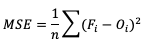
This measure has the same limits and perfect score as MAE, but squaring the differences does more than remove the sign of the differences: by squaring the error values, differences greater than one are penalized more severely than those that are less than one, with the penalty increasing at a squared rate. Using MSE, a forecast that over-forecasts temperature by two degrees from the observed value consistently over six time steps will have a smaller MSE than a forecast that over-forecasts temperature from the observed value by three degrees for three time steps and matched the observed value for the remaining three time steps.
The final error statistic to discuss is Root Mean Squared Error (RMSE). One of the most familiar statistical measures, RMSE is simply the square root of MSE, and has the same units as the forecasts and observations, providing an average error with a square-weight:
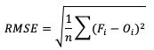
Similar to MSE, RMSE penalizes larger error magnitudes than smaller ones, and like MSE, RMSE provides no information on the sign (positive or negative) of the errors. It has the same range of values as MSE and a perfect forecast score would be an RMSE of zero. See how to use these statistics in METplus!
Standard Deviations
Unlike the family of mean error statistics, standard deviation focuses more on the individual groups of value sources; namely, the forecasts and observations. Standard deviations are a measure of how the variability of the values in a dataset differs from the average of their respective group. So keep in mind the general equation provided below can be applied to both observations and forecasts (and in some cases it may be meaningful to compare the standard deviation of the forecasts to the standard deviation of the observations):
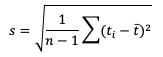
See how to use this statistic in METplus!
Multiplicative Bias
Like some of the other verification statistics for continuous forecasts, multiplicative bias (MBIAS) measures the ratio of the average forecast to the average observation. MBIAS is the ratio between these two averages, calculated using the following formula and has a range of all real numbers:
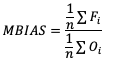
MBIAS has some of the same drawbacks as ME. In particular, MBIAS does not indicate the magnitudes of the forecast errors, which allows a perfect score of 1 to be achieved if the forecast errors compensate for each other (see the example for ME above for more information). It is recommended that any variable fields that utilize MBIAS contain all the same value signs (e.g. positive or negative) as mixing value signs together (for example, temperatures) would result in strange or unusable MBIAS results that included even more value compensation. See how to use this statistic in METplus!
Correlation Coefficients (Pearson, Spearman Rank, and Kendall’s Tau)
Because continuous forecasts and observations exist on the same real value spectrum, measurements of the linear association of the forecast-observation pairs create a vital foundation for verification statistics. Three measures of correlation (Pearson, Spearman Rank, and Kendall's Tau) measure this relationship in different ways.
Beginning with Pearson correlation coefficient, PR_CORR, the linear association of the forecast-observation pairs is measured using a sample covariance (e.g. the summed squared anomalies of two groups) and dividing by the product of the same two group’s standard deviations. In forecast verification, these two groups are the forecast and observation datasets and appear as
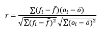
with r as the typical notation for the PR_CORR outside of METplus. From a visual perspective, PR_CORR measures the closeness of pairs of points, (i.e., representing the forecast and corresponding observation values) corresponding to a diagonal line. More generally these scatter plots can suggest the apparent relationship of any two variable fields, but for the purpose of this tutorial we will stay focused on the forecast-observation comparison. PR_CORR can range from negative one to positive one with either extreme of the range representing a perfect positive or negative linear association between the forecasts and observations. The PR_CORR remains sensitive to outliers and can produce a good correlation value for a poor forecast if that forecast has compensative errors.
Another way to estimate the linear association between forecasts and their corresponding observations involves ranking the forecast values when compared to the forecast group’s total range, do the same for the observation group, and then compute the correlation values. Spearman Rank correlation coefficient (SP_CORR) takes this approach while utilizing the same equation as PR_CORR. Because the rank values of both the forecast and observation datasets used to calculate SP_CORR are restricted to the integer values of 1 to n (the total number of matched forecast-observation pairs), the equation of SP_CORR can be simplified to
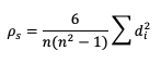
where di denotes the difference in ranking between the pair of datafields.
What does ranking of matched pairs look like with actual data? Let’s use the following scenario of rainfall forecasts and the observed rainfall over a five hour period for a set location:
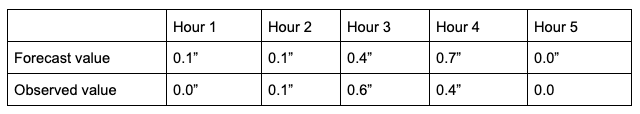
Using a ranking system for the datasets where 0.0” is assigned 1 and everything greater than that value is assigned a value that is integer-based, monotonically increasing by 1, the data table above would be transformed into the following ranks:
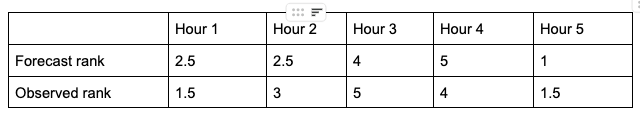
It is important that the forecast-observation pairs stay paired together, even when transformed into their rank values. Note the case when there is a tie in the ranks (i.e. a value appears more than once), all of the values receive the same average rank, keeping the total average rank for the number of values (in this scenario, five) consistent with the SP_CORR equation assumption. The next step is calculating the differences between the forecast ranks and the observed ranks, squaring the differences and summing them. After that, apply the rest of the equation and you should find ρ_s =0.825, a strong correlation value.
The Kendall’s Tau statistic (𝝉) is a variation on the SP_CORR equation ranking method. While all of the variable field values are ranked as was the case with SP_CORR, it’s the relationship between a pair of ranks and the pairs of ranks that follow, rather than the ranks within a given pair, that constitute 𝝉. To better understand, let’s first look at the equation for 𝝉:
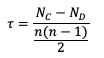
In the equation, N_C is a count of the concordant pairs, and N_D is a count of the discordant pairs. Simply put, a concordant pair is when a reference pair has rank values that are both larger or both smaller than a comparison pair. For example, consider the two pairs (3, 5) and (6, 8). Regardless of which pair is treated as the reference pair, the comparison pair will have both of the larger rank values (the case where (3, 5) is the reference pair) or both of the smaller rank values (the case where (6, 8) is the reference pair). A concordant pair is the complement to this: each pair in the comparison has one value that is bigger and one that is smaller. In the case of (3, 5) and (6, 2) the comparisons are considered discordant. In the case where the compared pairs are identical, there are multiple methods to choose: N_C and N_D can be incremented by ½ each, the tie can be ignored, or the tie can be penalized. For simplicity in counting, it is recommended to arrange one of the datasets in ascending or descending order (being careful to keep the matched pairs together) so that fewer comparisons need to be made.
To show how 𝝉 is calculated, let’s return to the previous example used to calculate SP_CORR. Because we’re using the same rainfall values, the rankings of those values will also be the same. For the simplicity of counting concordant and discordant pairs, the forecast ranks have been arranged in increasing order (which explains why Hour 5 is now proceeding Hour 1):
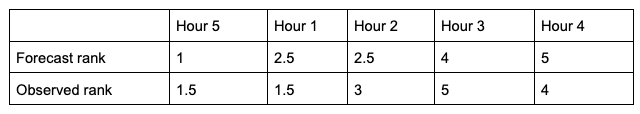
From this small change in the ordering, we see that two of the observed ranks do not increase (going from left to right): between Hour 5 and Hour 1 (they match at 1.5), and between Hour 3 and Hour 4 (5 compared to 4). Additionally, the forecast ranks between Hour 1 and Hour 2 do not increase (they match). In order to account for these ties, a “penalty” will be calculated using the following equation:
Where ti is the number of ranks that are involved in a given tie. Because both the forecast and observed ranks have a tie of two ranks, both will receive a Pt penalty of 2. As a result of this new handling of ties, an alternate form of 𝝉 sometimes referred to as 𝝉b must be used:
Using this slightly modified equation, we find a 𝝉b value of 0.56. As 𝝉 has the same range as SP_CORR (-1 to 1), a value of 0.56 shows some positive correlation between the two datasets. See how to use these statistics in METplus!
Anomaly Correlation
While similar to the traditional correlation coefficient, anomaly correlation is a somewhat different formulation: rather than directly comparing the pairs of forecast and observation values relative to the respective group averages, as is the case in PR_CORR, anomaly correlation is a measure of the deviations of forecast and observation values from climatological averages. Utilizing this third independent dataset for comparisons highlights any pattern of departures from the climatology, a correspondence of the forecast anomalies to the observed anomalies.
There are two widely used versions of anomaly correlation. The first is the centered anomaly correlation, which includes the mean error relative to the climatology. This version is calculated using

If it is not desirable to include the errors, the uncentered anomaly correlation is the better choice:

While there is an added effort required to find the matching climatology reference dataset for this statistic, it remains a highly resourceful statistic to use, especially with spatial verification, and is commonly used in operational forecasting centers. Anomaly correlation has a range from -1 to 1. See how to use this statistic in METplus!
METplus Solutions for Continuous Forecast Verification
METplus Solutions for Continuous Forecast Verification
METplus Solutions for Continuous Forecast Verification
Now that you know a bit more about continuous, deterministic forecasts and the related statistics, it’s time to show how you can access those same statistics in METplus!
Unsurprisingly METplus requires a slightly different approach to continuous variables and the thresholds that are used on these datasets. Rather than the cat_thresh arrays that are used for categorical variable fields, METplus uses cnt_thresh for filtering data prior to computing continuous statistics. Keep that in mind if you end up with a blank continuous line type file output; you may have not applied the correct thresholds!
In order to better understand the delineation between METplus, MET, and METplus wrappers which are used frequently throughout this tutorial but are NOT interchangeable, the following definitions are provided for clarity:
- METplus is best visualized as an overarching framework with individual components. It encapsulates all of the repositories: MET, METplus wrappers, METdataio, METcalcpy, and METplotpy.
- MET serves as the core statistical component that ingests the provided fields and commands to compute user-requested statistics and diagnostics.
- METplus wrappers is a suite of Python wrappers that provide low-level automation of MET tools and plotting capability. While there are examples of calling METplus wrappers without any underlying MET usage, these are the exception rather than the rule
MET Solutions
The MET User’s Guide provides an Appendix that dives into each and every statistical measure that it calculates, as well as the line type it is a part of. Statistics are grouped together by application and type and are available to METplus users in line types. For example, many of the statistics that were discussed above can be found in the Continuous Statistics (CNT) line type, which logically groups together statistics based on continuous variable fields.
For MET, which line types are output depends on your selection of the appropriate line type using the output_flag dictionary. Note that certain line types may or may not be available in every tool: for example, both Point-Stat and Grid-Stat produce CNT line types, which allows users access to the various continuous statistics for both point-based observations and gridded observations. But Ensemble-Stat is the only tool that can generate a Ranked Probability Score (RPS) line type which contains statistics relevant to the analysis of ensemble forecasts. If you don’t see your desired statistic in the line type or tool you’d expect it to be in, be sure to check the Appendix to see if the statistic is available in MET and which line type it’s currently grouped with.
As for the previous statistics that were discussed, here’s a link to the User’s Guide Appendix entry that discusses its use in MET:
- ME
- MAE
- MSE
- RMSE
- S (note that the linked s is for forecast; the observation s2 is just below it)
- MBIAS
- PR_CORR
- SP_CORR
- 𝝉 or KT_CORR
- ANOM_CORR
METplus Wrapper Solutions
The same statistics that are available in MET are also available with the METplus wrappers. To better understand how MET configuration options for statistics translate to METplus wrapper configuration options, you can utilize the Statistics and Diagnostics Section of the METplus wrappers User’s Guide, which lists all of the available statistics through the wrappers, including what tools can output what statistics. To access the line type through the tool, find your desired tool in the list of available commands for that tool. Once you do, you’ll see the tool will have several options that contain _OUTPUT_FLAG_. These will exhibit the same behavior and accept the same settings as the line types in MET’s output_flag dictionary, so be sure to review the available settings to get the line type output you want.
METplus Examples of Continuous Forecast Verification
METplus Examples of Continuous Forecast Verification
The following two examples show a generalized method for calculating continuous statistics: one for a MET-only usage, and the same example but utilizing METplus wrappers. These examples are not meant to be completely reproducible by a user: no input data is provided, commands to run the various tools are not given, etc. Instead, they serve as a general guide of one possible setup among many that produce continuous statistics.
If you are interested in reproducible, step-by-step examples of running the various tools of METplus, you are strongly encouraged to review the METplus online tutorial that follows this statistical tutorial, where data is made available to reproduce the guided examples.
In order to better understand the delineation between METplus, MET, and METplus wrappers which are used frequently throughout this tutorial but are NOT interchangeable, the following definitions are provided for clarity:
- METplus is best visualized as an overarching framework with individual components. It encapsulates all of the repositories: MET, METplus wrappers, METdataio, METcalcpy, and METplotpy.
- MET serves as the core statistical component that ingests the provided fields and commands to compute user-requested statistics and diagnostics.
- METplus wrappers is a suite of Python wrappers that provide low-level automation of MET tools and plotting capability. While there are examples of calling METplus wrappers without any underlying MET usage, these are the exception rather than the rule.
MET Example of Continuous Forecast Verification
Here is an example that demonstrates deterministic forecast verification in MET.
For this example, let’s examine two tools, PCP-Combine and Grid-Stat. Assume we wanted to verify a 6 hour period of precipitation forecasts over the continental United States. Using these tools, we will first combine the forecast files, which are hourly forecasts, into a 6 hour summation file with PCP-Combine. Then we will use Grid-Stat to place both datasets on the same verification grid and let MET calculate the continuous statistics available in the CNT line type. Starting with PCP-Combine, we need to understand what the desired output is first to know how to properly run the tool from the command line, as PCP-Combine does not use a configuration file. As stated previously, this scenario assumes the precipitation forecasts are hourly files and need to match the 6 hour observation file time summation. Of the four commands available in PCP-Combine, two seem to provide potential paths forward: sum and add.
While there are multiple methods that may work to successfully summarize the forecast files from these two commands, let’s assume that our forecast data files contain a time reference variable that is not CF-compliant {link to CF compliant time table in MET UG here}. As such, MET will be unable to determine the initialization and valid time of the files (without being explicitly set in the field array). Because the “add” command only relies on a list of files passed by the user to determine what is being summed, that is the command we will use.
With the information above, we construct the command line argument for PCP-Combine to be:
hrefmean_2017050912f018.nc \
hrefmean_2017050912f017.nc \
hrefmean_2017050912f016.nc \
hrefmean_2017050912f015.nc \
hrefmean_2017050912f014.nc \
hrefmean_2017050912f013.nc \
-field 'name="P01M_NONE"; level="(0,*,*)";' -name "APCP_06" \
hrefmean_2017051006_A06.nc
The command above displays the required arguments for PCP-Combine’s “add” command as well as an optional argument. When using the “add” command it is required to pass a list of the input files to be processed. In this instance we used a list of files, but had the option to pass an ASCII file that contained all of the files instead. Because each of the input forecast files contain the exact same variable fields, we utilize the “-field” argument to list exactly one variable field to be processed in all files. Alternatively we could have listed the same field information (i.e. 'name="P01M_NONE"; level="(0,*,*)";') after each input file. Finally, the output file name is set to “hrefmean_2017051006_A06.nc”, which contains references to the valid time of the file contents as well as how many hours the precipitation is accumulated over. The optional argument “-name” sets the output variable field name to “APCP_06”, following GRIB standard practices.
After a successful run of PCP-Combine we now have a six hour accumulation field forecast of precipitation and are ready to set our Grid-Stat configuration file. Starting with the general Grid-Stat configuration file {provide link here}, the following would resemble minimum necessary settings/changes for the fcst and obs dictionaries:
field = [
{
name = "APCP_06";
level = [ "(*,*)" ];
}
];
}
obs = {
field = [
{
name = “P06M_NONE”;
level = [“(@20170510_060000,*,*)”];
}
];
}
Both input files are netCDF format and so require the asterisk and parentheses method of level access. The observation input file level required a third dimension as more than one observation time is available. We used the “@” symbol to take advantage of MET’s ability to parse time dimensions by the user-desired time, which in this case was the verification time. Note how the variable field name that was set in PCP-Combine’s output file is used in the forecast field information. Because the two variable fields are not on the same grid, an independent grid is chosen as the verification grid. This is set using the in-tool method for regridding:
to_grid = "CONUS_HRRRTLE.nc";
…
Now that the verification is being performed on our desired grid and the variable fields are set to be read in, all that’s left in the configuration file is to set the output. This time, we’re interested in the CNT line type and set the output flag library accordingly:
fho = NONE;
ctc = NONE;
cts = NONE;
mctc = NONE;
mcts = NONE;
cnt = STAT;
sl1l2 = NONE;
…
And as a sanity check we can see the input fields the way MET is ingesting them by selecting the desired nc_pairs_flag library settings:
latlon = TRUE;
raw = TRUE;
diff = TRUE;
climo = FALSE;
climo_cdp = FALSE;
seeps = FALSE;
weight = FALSE;
nbrhd = FALSE;
fourier = FALSE;
gradient = FALSE;
distance_map = FALSE;
apply_mask = FALSE;
}
All that’s left is to run MET with a command line prompt:
The resulting two files have a wealth of information and statistics. The netCDF output contains our visual confirmation that the forecast and observation input fields were interpreted correctly by MET, as well as the difference between the two fields which is provided below:
For the CNT line type output we review the .stat file and find something similar to the following:
The columns that are available in the CNT line type are listed in the MET User’s Guide guidance for CNT line type {provide link here}. After the declaration of the line type (CNT), the familiar TOTAL or matched pairs column, we find a wealth of statistics including the forecast and observation means, the forecast and observation standard deviations, ME, MSE, along with all of the other statistics discussed in this section, all with their appropriate lower and upper confidence intervals and the bootstrap confidence intervals. Note that because the bootstrap library’s n_rep variable was kept at its default value of 0, bootstrap methods were not used and appear as NA in the stat file. You’ll also note that the ranking statistics (SP_CORR and KT_CORR) are listed as NA because we did not set rank_corr_flag to TRUE in the Grid-Stat configuration file. This was done intentionally; in order to calculate ranking statistics MET needs to assign each and every matched pair a rank and then perform the calculations. With a large dataset with numerous matched pairs this can significantly increase runtime and be computationally intensive. Given our example had over 1.5 million matched pairs, these statistics are best left to a smaller domain. Let’s create that smaller domain in a METplus wrappers example!
METplus Wrapper Example of Continuous Forecast Verification
To achieve the same success as the previous example but utilizing METplus wrappers instead of MET, very few adjustments would need to be made. Because METplus wrappers have the helpful feature of chaining multiple tools together, we’ll start off by listing all of the tools we want to use. Recall that for this example, we want to include a smaller verification area to enable the rank correlation statistics as well. This results in the following process list:
The second listing of GridStat uses the instance feature to allow a second run of Grid-Stat with different settings. Now we need to set the _VAR1 settings appropriately:
FCST_VAR1_LEVELS = "(*,*)"
OBS_VAR1_NAME = P06M_NONE
OBS_VAR1_LEVELS = "({valid?fmt=%Y%m%d_%H%M%S},*,*)"
We’ve utilized a different setting, FCST_PCP_COMBINE_OUTPUT_NAME, to control what forecast variable name is verified. This way if a different forecast variable were to be used in a later run (assuming it had the same level dimensions as the precipitation), the forecast variable name would only need to be changed in one place instead of multiple. We also utilize METplus wrappers' ability to set an index based on a time, behaving similarly to the “@” usage in the MET example. Now we need to create all of the settings for PCPCombine:
<\br> FCST_PCP_COMBINE_INPUT_DATATYPE = NETCDF
FCST_PCP_COMBINE_CONSTANT_INIT = true
FCST_PCP_COMBINE_INPUT_ACCUMS = 1
FCST_PCP_COMBINE_INPUT_NAMES = P01M_NONE
FCST_PCP_COMBINE_INPUT_LEVELS = "(0,*,*)"
FCST_PCP_COMBINE_OUTPUT_ACCUM = 6
FCST_PCP_COMBINE_OUTPUT_NAME = APCP_06
From these settings, we see that all of the arguments from the command line for PCP-Combine are present: we will use the “add” method to loop over six netCDF files, each containing a variable field name of P01M_NONE and accumulation times of one hour. The output variable should be named APCP_06 and will be stored in the location as directed by FCST_PCP_COMBINE_OUTPUT_DIR and FCST_PCP_COMBINE_OUTPUT_TEMPLATE (not shown above).
Because the loop/timing information is controlled inside the configuration file for METplus wrappers (as opposed to MET’s non-looping option), that information must also be set accordingly, paying close attention that both instances of GridStat and PCPCombine will behave as expected:
INIT_TIME_FMT = %Y%m%d%H
INIT_BEG=2017050912
INIT_END=2017050912
INIT_INCREMENT=12H
LEAD_SEQ = 18
Recall that we need to perform the verification on an alternate grid for one of the instances, and a small subset of the larger area in the other. So in the first instance configuration file area (anywhere outside of the [rank] instance configuration file area) we add
GRID_STAT_REGRID_METHOD = NEAREST
And set the [rank] instance up as follows:
GRID_STAT_REGRID_TO_GRID = 'latlon 40 40 33.0 -106.0 0.1 0.1'
GRID_STAT_MET_CONFIG_OVERRIDES = rank_corr_flag = TRUE;
GRID_STAT_OUTPUT_TEMPLATE = {init?fmt=%Y%m%d%H%M}_rank
For this instance of GridStat, we’ve set our own verification area using the grid definition option {link grid project here}, and utilized the OVERRIDES option {link to the OVERRIDES discussion here} to set the rank_corr_flag option, which is currently not a METplus wrapper option, to TRUE. Because both GridStat instances will create CNT output, the [rank] instance CNT output would normally overwrite the first GridStat instance. To avoid this, we create a new output template for the [rank] instance of GridStat to follow, preserving both files.
Finally, the desired line types and nc_pairs_flag settings need to be selected for output. This can be done outside of the [rank] instance, as any setting that is not overwritten by an instance further down the configuration file will be propagated to all applicable tools in the configuration file:
GRID_STAT_NC_PAIRS_FLAG_LATLON = TRUE
GRID_STAT_NC_PAIRS_FLAG_RAW = TRUE
GRID_STAT_NC_PAIRS_FLAG_DIFF = TRUE
With a proper setting of the input and output directories, file templates, and a successful run of METplus, the same .stat output and netCDF file that were created in the MET example would be produced here, complete with CNT line type. However this example would result in two additional files: one .stat file that contains values for the rank correlation statistics and a netCDF file with the smaller area that was used to calculate them. The contents of that second .stat file would look something like the following:
We can see the smaller verification area resulted in only 1,600 matched pairs, which is much more reasonable for rank computations. SP_CORR was 0.41127 showing a positive correlation, while KT_CORR was 0.28929, a slightly weaker positive correlation. METplus goes the additional step and also shows that of the 1,600 ranks that were used to calculate KT_CORR, it found 1,043 forecast ranks that were tied and 537 observation ranks that were tied. Not something that would be easily computed without the help of METplus!
Probabilistic Forecasts
Probabilistic Forecasts
Probabilistic Forecasts
When reviewing the other forecast types in this tutorial, you’ll notice that all of them are deterministic (i.e., non-probabilistc) values. They have a quantitative value that can be verified with observations. Probabilistic forecasts on the other hand, do not provide a specific value relating directly to the variable (precipitation, wind speed, etc.). Instead, probabilistic forecasts provide, you guessed it, a probability of a certain event occurring. The most common probabilistic forecasts are for precipitation. Given the spatial and temporal irregularities any precipitation type could display during accumulation, probabilities are a better option for numerical models to provide for the general public. It allows the general public to decide for themselves if a 60% forecasted chance of rain is enough to warrant bringing an umbrella to the outdoor event, or if a 40% forecasted chance of snow is too much to consider going for a long hike. Consider the alternative where deterministic forecasts were used for precipitation: would it be more beneficial to hear a forecast of no precipitation for any probability less than 20% and precipitation forecasted for anything greater than 20% (i.e. a categorical forecast)? Or maybe a scenario where the largest amount of precipitation is presented as the precipitation a given area will experience with no other information (i.e. a continuous forecast)? While they have other issues which will be explored in this section, probabilistic forecasts play an important part in weather verification statistics. Moreover, they require special measures for verification.
Verification Statistics for Probabilistic Forecasts
Verification Statistics for Probabilistic Forecasts
Verification Statistics for Probabilistic Forecasts
The forecast types we’ve examined so far focused on dichotomous predictions of binary events (e.g.,. the tornado did or did not happen and the forecast did or did not predict the event); application of one or more thresholds; or specification of the value itself for the forecasted event (e.g.,. the observed temperature compared to a forecast of 85 degrees Fahrenheit). These forecast types determined how the verification statistics were calculated. But how are probabilistic datasets handled? When there is an uncertainty value attached to a meteorological event, what statistical measures can be used?
A common method to avoid dealing directly with probabilities is to convert forecasts from probabilistic space into deterministic space using a threshold. Consider an example rainfall forecast where the original forecast field is issued in tens values of probability (0%, 10%, 20% ... 80%, 90%, 100%). This could be converted to a deterministic forecast by establishing a threshold such as “the probability of rainfall will exceed 60%”. This threshold sets up a binary forecast (probabilities at or below 60% are “no” and probabilities above 60% are “yes”) and two separate observation categories (rain was observed or rain did not occur) that all of the occurrences and non-occurrences can be placed in. While the ability to access categorical statistics and scores is an obvious benefit to this approach, there are clear drawbacks to this method. The loss of probability information tied to the particular forecast value removes an immensely useful aspect of the forecast. As discussed previously, the general public may desire probability space information to make their own decisions: after all, what if someone’s tolerance for rainfall is lower than the 60% threshold used to calculate the statistics (e.g., the probability of rainfall will exceed 30%)?
Brier Score
One popular score for probability forecasts is the Brier Score (BS). Effectively a Mean Squared Error calculation, it is a scalar value of forecast accuracy that conveys the magnitude of the probability errors in the forecast.
Here, pi is the forecast probability while oi is the binary representation of the observance of the event (1 if the event occurred, 0 if the event did not occur). This summation score is negatively oriented, with a 0 indicating perfect accuracy and 1 showing complete inaccuracy. The score is sensitive to the frequency of an event and should only be used on forecast-observation datasets that boast a substantial number of event samples.
Through substitutions, BS can be decomposed into three terms that describe the reliability, resolution, and uncertainty of the forecasts (more on these attributes can be found in the Attributes of Forecast Quality section). This decomposition is given as
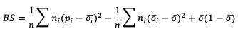
where the three terms are reliability, resolution, and uncertainty, respectively. ni is the count of probabilistic forecasts that fall into each probabilistic bin. See how to use this statistic in METplus!
Ranked Probability Score
A second statistical score to use for probabilistic forecasts is the Ranked Probability Score (RPS). This score differs from BS in that it allows the verification of multicategorical probabilistic forecasts where BS strictly pertains to binary probabilistic forecasts. While the RPS formula is based on a squared error at its core (similar to BS), it remains sensitive to the distance between the forecast probability and the observed event space (1 if the event occurred, 0 if it did not) by calculating the squared errors in cumulative probabilistic forecast and observation space. This formulation is represented in the following equation
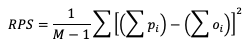
Note how RPS reduces to BS when there are only two forecast categories evaluated. In the equation, M denotes the number of categories the forecast is divided into. Because of the squared error usage, RPS is negative orientated with a 0 indicating perfect accuracy and 1 showing complete inaccuracy. See how to use this statistic in METplus!
Continuous Ranked Probability Score
Similar to the RPS’s approach to provide a probabilistic evaluation of multicategorical forecasts and the BS formulation as a statistic for binary probabilistic forecasts, the Continuous Ranked Probability Score (CRPS) provides a statistical measure for forecasts in the continuous probabilistic space. Theoretically this is equivalent to evaluating multicategorical forecasts that extend across an infinite number of categories that are infinitesimally small. When it comes to application, however, it becomes difficult to express mathematically a closed form of CRPS. Due to this restriction, CRPS often utilizes an assumption of a Gaussian (i.e. normal) distribution in the dataset and is presented as
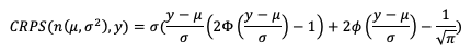
In this equation we use μ and σ to denote the mean and standard deviation of the forecasts, respectively, ɸ to represent the cumulative distribution function (CDF ) and 𝚽 to represent the probability density function (PDF) of the normal distribution. If you’ve previously evaluated meteorological forecasts, you know that the assumption that the dataset can be described by a Gaussian distribution is not always correct. Temperature and pressure variable fields, among others, can usually take advantage of this CRPS definition as they often are well fitted by a Gaussian distribution. But other important meteorological fields, such as precipitation, do not. Using statistics that are created with an incorrect assumption will produce, at best, misleading results. Be sure that your dataset follows a Gaussian distribution before relying on the above definition of CRPS!
The CRPS is negatively oriented with a 0 indicating perfect accuracy and 1 showing complete inaccuracy. See how to use this statistic in METplus!
Probabilistic Skill Scores
Probabilistic Skill Scores
Probabilistic Skill Scores
Some of the previously mentioned verification statistics for probabilistic forecasts can be used to compute skill scores that are regularly used. All of these skill scores use the same general equation format of comparing their respective score results to a base or reference forecast, which can be climatology, a “random” forecast, or any other comparison that could provide useful information.
Brier Skill Score
The Brier Skill Score (BSS) measures the relative skill of the forecast compared to a reference forecast. It’s equation is simple and follows the general skill score format:
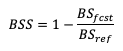
Compared to the BS equation, the range of values for BSS differs: the range is from negative infinity to 1, with 1 showing a perfect skill and 0 showing no discernable skill compared to a reference forecast. See how to use this skill score in METplus!
Ranked Probability Skill Score
Similar to the BSS, the Ranked Probability Skill Score (RPSS) follows the general skill score equation formulation, allowing a comparison between a chosen reference forecast and the forecast of interest:
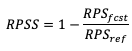
RPSS measures the improvement/degradation of the ranked probability forecasts compared to the skill of a reference forecast. As with BSS, RPSS ranges from negative infinity to 1, with a perfect score of 1, and a score of zero indicating no improvement of forecast performance relative to the reference forecast. See how to use this skill score in METplus!
METplus Solutions for Probabilistic Forecast Verification
METplus Solutions for Probabilistic Forecast Verification
METplus Solutions for Probabilistic Forecast Verification
If you utilize METplus verification capabilities to evaluate probabilistic forecasts, you may find that your final statistical values are not exactly the same as when you compute the same statistic by pencil and paper or in a separate statistical program. These very slight differences are due to how METplus handles probabilistic information.
MET is coded to utilize categorical forecasts, creating contingency tables and using the counts in each of the contingency table cells (hits, misses, false alarms, and correct rejections) to calculate the desired verification statistics. This use extends to probabilistic forecasts as well and aids in the decomposition of statistics such as Brier Score (BS) into reliability, resolution, and uncertainty (more information on that decomposition can be found here).
MET requires users to provide three conditions for probabilistic forecasts. The first of these conditions is an observation variable that is either a 0 or 1 and a forecast variable that is defined on a scale from 0 to 1. In MET, this boolean is prob and METplus Wrappers utilizes the variable FCST_IS_PROB. In MET prob can also be defined as a dictionary with more information on how to process the probabilistic field; please review this section of the User’s Guide for information.
The second condition is the thresholds to evaluate the probabilistic forecasts across. Essentially this is where METplus turns the forecast probabilities into a binned, categorical evaluation. At its most basic usage in a MET configuration file, this looks like
cat_thresh = ==0.1;
which would create 10 bins of equal width. Users have multiple options for setting this threshold and should review this section of the User’s Guide for more information. It’s important to note that when it comes to evaluating a statistic like BS, METplus does not actually use the forecasts’ probability value; instead, it will use the midpoint of the bin width between the thresholds for the probabilistic forecasts. To understand what this looks like in METplus, let's use the previous example where 10 bins of equal width were created. When calculating BS, METplus will evaluate the first probability bin as 0.05, the midway point between the first bin (0.0 to 0.1). The next probability value would be 0.15 (the midway point between 0.1 and 0.2), and so on. MET utilizes an equation of BS that is described in more detail in the MET Appendix which evaluates to the same result as the BS equation provided in the Verification Statistics for Probabilistic Forecasts section of this guide {provide link to previous section here} if the midpoints of the bins are used as the probability forecast values. All of this is to stress that a proper selection of bin width (and the accompanying mid-point of those bins) will ultimately determine how meaningful your resulting BS value is; after all, what would the result be if the midpoint of a bin was 0.1 and many of the forecasts values were 0.1? What contingency table bin will they count towards?
The final condition users need to provide to MET for probabilistic forecasts is a threshold for the observations. As alluded to in the second condition, users can create any number of thresholds to evaluate the probabilistic forecasts. Combined with the observation threshold which determines an event observation from non-event observation, an Nx2 contingency table will be created, where N is the number of probabilistic bins for the forecasts and 2 is the event, non-event threshold set on the observations.
Now that you know a bit more about probabilistic forecasts and the related statistics as well as how MET will process them, it’s time to show how you can access those same statistics in METplus!
In order to better understand the delineation between METplus, MET, and METplus wrappers which are used frequently throughout this tutorial but are NOT interchangeable, the following definitions are provided for clarity:
- METplus is best visualized as an overarching framework with individual components. It encapsulates all of the repositories: MET, METplus wrappers, METdataio, METcalcpy, and METplotpy.
- MET serves as the core statistical component that ingests the provided fields and commands to compute user-requested statistics and diagnostics.
- METplus wrappers is a suite of Python wrappers that provide low-level automation of MET tools and plotting capability. While there are examples of calling METplus wrappers without any underlying MET usage, these are the exception rather than the rule.
MET solutions
The MET User’s Guide provides an Appendix that dives into statistical measures that it calculates, as well as the line type it is a part of. Statistics are grouped together by application and type and are available to METplus users in line types. For the probabilistic-related statistics discussed in this section of the tutorial, MET provides the Contingency Table Counts for Probabilistic forecasts (PCT) line type, and the Contingency Table Statistics for Probabilistic forecasts (PSTD) line types. The PCT line type is critical for checking if the thresholds for the probabilistic forecasts and observations produced contingency table counts that reflect what the user is looking for in probabilistic verification. Remember that these counts are ultimately what determine the statistical values found in the PSTD line type.
As for the statistics that were discussed in the Verification Statistics section, the following are links to the User’s Guide Appendix entry that discusses their use in MET. Note that Continuous Ranked Probability Score (CRPS) and Continuous Ranked Probability Skill Score (CRPSS) appear in the Ensemble Continuous Statistics (ECNT) line type and can only be calculated from the Ensemble-Stat tool, while Ranked Probability Score (RPS) and Ranked Probability Skill Score (RPSS) appear in their own Ranked Probability Score (RPS) line type output that is also only accessible from Ensemble-Stat. RPSS is not discussed in the MET USer’s Guide Appendix and is not linked below, while discussion of CRPSS is provided to users in the existing documentation in the MET User’s Guide Appendix:
METplus Wrapper Solutions
The same statistics that are available in MET are also available with the METplus wrappers. To better understand how MET configuration options for statistics translate to METplus wrapper configuration options, you can utilize the Statistics and Diagnostics Section of the METplus wrappers User’s Guide, which lists all of the available statistics through the wrappers, including what tools can output what statistics. To access the line type through the tool, find your desired tool in the list of available commands for that tool. Once you do, you’ll see the tool will have several options that contain _OUTPUT_FLAG_. These will exhibit the same behavior and accept the same settings as the line types in MET’s output_flag dictionary, so be sure to review the available settings to get the line type output you want.
METplus Examples of Probabilistic Forecast Verification
METplus Examples of Probabilistic Forecast Verification
METplus Examples of Probabilistic Forecast Verification
The following two examples show a generalized method for calculating probabilistic statistics: one for a MET-only usage, and the same example but utilizing METplus wrappers. These examples are not meant to be completely reproducible by a user: no input data is provided, commands to run the various tools are not given, etc. Instead, they serve as a general guide of one possible setup among many that produce probabilistic statistics.
If you are interested in reproducible, step-by-step examples of running the various tools of METplus, you are strongly encouraged to review the METplus online tutorial that follows this statistical tutorial, where data is made available to reproduce the guided examples.
In order to better understand the delineation between METplus, MET, and METplus wrappers which are used frequently throughout this tutorial but are NOT interchangeable, the following definitions are provided for clarity:
- METplus is best visualized as an overarching framework with individual components. It encapsulates all of the repositories: MET, METplus wrappers, METdataio, METcalcpy, and METplotpy.
- MET serves as the core statistical component that ingests the provided fields and commands to compute user-requested statistics and diagnostics.
- METplus wrappers is a suite of Python wrappers that provide low-level automation of MET tools and plotting capability. While there are examples of calling METplus wrappers without any underlying MET usage, these are the exception rather than the rule.
MET Example of Probabilistic Forecast Verification
Here is an example that demonstrates probabilistic forecast verification using MET.
For this example, we will use two tools: Gen-Ens-Prod, which will be used to create uncalibrated probability forecasts, and Grid-Stat, which will verify the forecast probabilities against an observational dataset. The “uncalibrated” term means that the probabilities gathered from Gen-Ens-Prod may be biased and will not perfectly reflect the true probabilities of the forecasted event. To avoid complications with assuming gaussian distributions on non-gaussian variable fields (i.e. precipitation), we’ll verify the probability of a CONUS 2 meter temperature field from a global ensemble with 5 members with a threshold of greater than 10 degrees Celsius.
Starting with the general Gen-Ens-Prod configuration file, the following would resemble the minimum necessary settings/changes for the ens dictionary:
ens_thresh = 0.3;
vld_thresh = 0.3;
convert(x) = K_to_C(x)
field = [
{
name = "TMP";
level = “Z2";
cat_thresh = [ >10 ];
}
];
}
We can see right away that Gen-Ens-Prod is different from most MET tools; it utilizes only one dictionary to process fields (as opposed to the typical forecast and observation fields). This is by design and follows the guidance that Gen-Ens-Prod generates ensemble products, rather than verifying ensemble forecasts (which is left for Ensemble-Stat). Even with this slight change, the name and level entries are still set the same as they would be in any MET tool; that is, according to the information in the input files (e.g., a variable field named TMP on the second vertical level). The cat_thresh entry reflects an interest in 2 meter temperatures greater than 10 degrees Celsius. We’ve also included a convert function which will convert the field from its normal output of Kelvin to degrees Celsius. If you’re interested in learning more about this tool, including in-depth explanations of the various settings, please review the MET User’s Guide entry for Gen-Ens-Prod or get a hands-on experience with the tool in the METplus online tutorial.
Let’s also utilize the regrid dictionary, since we are only interested in CONUS and the model output is global:
to_grid = "G110";
method = NEAREST;
width = 1;
vld_thresh = 0.5;
shape = SQUARE;
}
More discussion on how to properly use the regrid dictionary and all of its associated settings can be found in the MET User’s Guide.
All that’s left before running the tool is to set up the ensemble_flag dictionary correctly:
latlon = TRUE;
mean = FALSE;
stdev = FALSE;
minus = FALSE;
plus = FALSE;
min = FALSE;
max = FALSE;
range = FALSE;
vld_count = FALSE;
frequency = TRUE;
nep = FALSE;
…
In the first half of this example, we have told MET to create a CONUS 2 meter temperature field count from 0.0 to 1.0 at each grid point representing how many of the ensemble members forecast a temperature greater than 10 degrees Celsius. So with this configuration file we’ll create a probability field based on ensemble member agreement and disagreement.
The output from Gen-Ens-Prod is a netCDF file whose content would contain a variable field as described above. It should look something like the following:
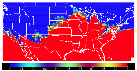
With this new MET field output, we can verify this uncalibrated probabilistic forecast for 2 meter temperatures greater than 10 degrees Celsius against an observation dataset in Grid-Stat.
Now for the actual verification and statistical generation we turn to Grid-Stat. Starting with the general Grid-Stat configuration file, let’s review how we might set the fcst dictionary:
field = [
{
name = "TMP_Z2_ENS_FREQ_gt10";
level = [ "(*,*)" ];
prob = TRUE;
cat_thresh = [ ==0.1 ];
}
];
}
In this example we see the name of the variable field from the Gen-Ens-Prod tool’s netCDF output file, TMP_Z2_ENS_FREQ_gt10, set as the forecast field name. The prob setting informs MET to process the field as probabilistic data, which requires an appropriate categorical threshold creation. Using “==0.1” means MET will create 10 bins from 0 to 1, each with a width of 0.1. Recall from previous discussion on how MET evaluates probabilities that MET will use the midpoints of each of these bins to evaluate the forecast. Since the forecast data probabilistic resolution is 0.1, the use of 0.05 as the evaluation increment is reasonable.
Now let’s look at a possible setup for the obs dictionary:
field = [
{
convert(x) = K_to_C(x);
name = "TMP";
level = "Z2";
cat_thresh = [>10];
}
Notice that we’ve used the convert function again to change the original Kelvin field to degrees Celsius, along with the appropriate variable field name and second vertical level request. For the threshold we re-use the same value that was originally used to create the forecast probabilities, greater than 10 degrees Celsius. This matching value is important as any other comparison would mean an evaluation between two inconsistent fields.
Since the forecast and observation fields are on different grids, we’ll utilize the regrid dictionary once again to place everything on the same evaluation gridspace:
to_grid = FCST;
method = NEAREST;
width = 1;
vld_thresh = 0.5;
shape = SQUARE;
}
Finally, we choose the appropriate flags in the output_flag dictionary to gain the probabilistic statistics:
pct = STAT;
pstd = STAT;
…
With a successful run of MET, we should find a .stat file with two rows of data; one for the PCT line type that will provide information on the specific counts of observations that fell into each of the forecast’s probability bins, and one for the PSTD line type which has some of the probabilistic measures we discussed in this chapter. The content might look similar to the following:
Note that the rows have been truncated and would normally hold more information to the left of the FCST_THRESH entry. But from this snippet we see that there were 103,936 matched pairs for the comparison, with PCT line type showing many of the observations falling in the “no” category of the 0 to 0.1 bin and the “yes” category of the 0.9 to 1.0 bin. In fact, less than seven percent of the matched pairs fell into categories outside of these two. This distribution tells us that the model was very confident in its probabilities, supported by the observations. This is reflected in the outstanding statistical values of the PSTD line type, including a 0.0019261 Reliability value (recall that a zero is ideal and indicates less differences between the average forecast probability and the observed average frequency) and a near-perfect Brier score of 0.019338 (0 being a perfect score). There is some room for improvement, as reflected in a 0.231 Resolution value (remember that this is the measure of the forecast’s ability to resolve different observational distributions given a change in the forecast value, and a larger value is desirable). For a complete list of all of the statistics given in these two line types, review the MET User’s Guide entries for the PCT and PSTD line types.
METplus Wrapper Example of Probabilistic Forecast Verification
To achieve the same success as the previous example, but utilizing METplus wrappers instead of MET, very few adjustments would need to be made. In fact, approaching this example utilizing the wrappers simplifies the problem, as one configuration file can be used to generate the desired output from both tools.
Starting with variable fields, we would need to set the _VAR1 settings appropriately. Since we are calling two separate tools, it would be best practice to utilize the individual tool’s variable field settings, as seen below:
ENS_VAR1_LEVELS = Z2
ENS_VAR1_OPTIONS = convert(x) = K_to_C(x);
ENS_VAR1_THRESH = >10
GEN_ENS_PROD_ENS_THRESH = 0.3
GEN_ENS_PROD_VLD_THRESH = 0.3
FCST_GRID_STAT_VAR1_NAME = TMP_Z2_ENS_FREQ_gt10
FCST_GRID_STAT_VAR1_LEVELS = “(*,*)”
FCST_GRID_STAT_VAR1_THRESH = ==0.1
FCST_GRID_STAT_IS_PROB = True
OBS_GRID_STAT_VAR1_NAME = TMP
OBS_GRID_STAT_VAR1_LEVELS = Z2
OBS_GRID_STAT_VAR1_THRESH = >10
OBS_GRID_STAT_VAR1_OPTIONS = convert(x) = K_to_C(x);
You can see how the GenEnsProd field variables start with the prefix ENS_, and the GridStat wrapper field variables have _GRID_STAT_ in their name. Those GridStat field settings are also clearly separated into forecast (FCST_) and observation (OBS_) options. Note how from the MET-only approach we have simply changed what the setting name is, but the same values are utilized, all in one configuration file.
To recreate the regridding aspect of the MET example, we would call the wrapper-appropriate regridding options:
GEN_ENS_PROD_REGRID_TO_GRID = “G110”;
Because the loop/timing information is controlled inside the configuration file for METplus wrappers (as opposed to MET’s non-looping option), that information must also be set accordingly. This is also an appropriate time to set up the calls to the wrappers in the desired order:
LOOP_BY = INIT
INIT_TIME_FMT = %Y%m%d%H
INIT_BEG=2024030300
INIT_END=2024030300
INIT_INCREMENT = 12H
LEAD_SEQ = 24
Now a one time loop will be executed with a forecast lead time of 24 hours, matching the forecast and observation datasets’ relationship.
One part that needs to be done carefully is the input directory and file name template for GridStat. This is because we are relying on the output from the previous wrapper, GenEnsProd, and need to set the variable accordingly. As long as the relative value is used, this process becomes much simpler, as shown:
FCST_GRID_STAT_INPUT_TEMPLATE = {GEN_ENS_PROD_OUTPUT_TEMPLATE}
These commands will tie the input for GridStat to wherever the output from GenEnsProd was set.
Finally we set up the correct output requests for each of the tools:
GEN_ENS_PROD_ENSEMBLE_FLAG_FREQUENCY = TRUE
GRID_STAT_OUTPUT_FLAG_PSTD = STAT
GRID_STAT_OUTPUT_FLAG_PCT = STAT
And with a successful run of METplus we would arrive at the same output as we obtained from the MET-only example. This example once again highlights the usefulness of METplus wrappers in chaining multiple tools together in one configuration file.
Preliminary work: METplus setup
Preliminary work: METplus setup
Welcome to the online METplus tutorial!
In this preliminary session, you'll be guided through the necessary steps that need to happen before executing the tutorial's METplus commands. Additionally, we'll go over some of the common METplus wrapper configuration settings, timing control, and the directory structure of the METplus wrappers.
If you have already started working on the tutorial and are rejoining with the same METplus terminal session active (i.e. you have not changed any of the environmental configuration settings), you do not need to redo this section and can jump directly to the session of interest.
If you are just starting out, or you are returning with a new terminal session, you will need to revisit this session to get your environment correctly set. So select the next page of "METplus setup" to get started!
METplus Setup
METplus Setup
METplus Overview
METplus is a set of Python modules that have been developed with the flexibility to run the MET applications for various use cases or scenarios. The goal is to simplify the running of MET for scientists. Currently, the primary means of achieving this is through the use of METplus configuration files, aka "conf files." It is designed to provide a framework in which additional use cases can be added. The conf file implementation utilizes a Python package called produtil that was developed by NOAA/NCEP/EMC for the HWRF system.
Please be sure to follow the instructions in order.
METplus Useful Links
The following links are just for reference, and not required for this practical session. METplus releases are available on GitHub along with sample data and instructions.
The source code for the METplus components are publicly available in the following GitHub repositories:
- https://github.com/dtcenter/METplus - Python wrappers and use cases
- https://github.com/dtcenter/MET - Core MET codebase
- https://github.com/dtcenter/METdataio - Database system for MET output
- https://github.com/dtcenter/METplotpy - Python plotting scripts
- https://github.com/dtcenter/METcalcpy - Python calculation functions
- https://github.com/dtcenter/METviewer - Display system for MET output
- https://github.com/dtcenter/METexpress - Streamlined display system
New features are developed and bugs are tracked using GitHub issues in each repository.
METplus: Initial setup
METplus: Initial setup
Prerequisites: Software
The Requirements section in the Software Installation chapter of the METplus User's Guide lists the software and Python packages that are required to run the METplus wrappers. Note that there is a core set of requirements needed to run the METplus wrappers and additional requirements needed to utilize some of the more advanced features.
Prerequisites: Environment
The following instructions are required so the commands in this tutorial can be copied and run without modification. The steps involve creating a working directory to store files used/generated by the tutorial and configuring a simple script that can be run to set up the shell environment. Once configured correctly, the script can be run upon returning to the tutorial content to easily resume progress.
Pre-Configured Environments
Setting up the Tutorial Environment on Hera (NOAA)
Setting up the Tutorial Environment on Jet (NOAA)
Setting up the Tutorial Environment on Cheyenne (NCAR)
Setting up the Tutorial Environment on Seneca (NCAR)
User Configured Environments
Setting up the Tutorial Environment (bash)
Setting up the Tutorial Environment (csh)
Setting up the Tutorial Environment on Cheyenne (NCAR)
Setting up the Tutorial Environment on Cheyenne (NCAR)
Setting up the Tutorial Environment on Cheyenne (NCAR)
The following instructions should be run if configuring the shell environment to run the METplus Tutorial on Cheyenne (NCAR). If you are running on your own computer or a NOAA machine that has been set up to run the tutorial, please go back and click the appropriate link for those instructions.
Create a Working Directory
Create a directory called 'METplus-5.0.0_Tutorial' to hold all of the files you will create during the tutorial. This can be any directory that you have write permission.
Create Directories for Configuration Files and Output Data
mkdir output
Obtain the Tutorial Setup Script
DO NOT RUN BOTH SETS OF COMMANDS.
If you are unsure which shell you are using, run the command "echo $SHELL" to check.
Setting up the Tutorial Environment on Jet (NOAA)
Setting up the Tutorial Environment on Jet (NOAA)
Setting up the Tutorial Environment on Jet (NOAA)
The following instructions should be run if configuring the shell environment to run the METplus Tutorial on Jet (NOAA). If you are running on your own computer or an NCAR machine that has been set up to run the tutorial, please go back and click the appropriate link for those instructions.
Create a Working Directory
Create a directory called 'METplus-5.0.0_Tutorial' to hold all of the files you will create during the tutorial. This can be any directory that you have write permission.
Create Directories for Configuration Files and Output Data
mkdir output
Obtain the Tutorial Setup Script
cp /lfs1/HFIP/dtc-hurr/METplus/METplus-5.0.0_Tutorial_Files/tutorial-5.0.0.conf ./tutorial.conf
Setting up the Tutorial Environment on Seneca (NCAR)
Setting up the Tutorial Environment on Seneca (NCAR)
Setting up the Tutorial Environment on Seneca (NCAR)
The following instructions should be run if configuring the shell environment to run the METplus Tutorial on Seneca (NCAR). If you are running on your own computer or a NOAA machine that has been set up to run the tutorial, please go back and click the appropriate link for those instructions.
Create a Working Directory
Create a directory called 'METplus-5.0.0_Tutorial' to hold all of the files you will create during the tutorial. This can be any directory that you have write permission.
Create Directories for Configuration Files and Output Data
mkdir output
Obtain the Tutorial Setup Script
(OPTIONAL) Set up conda Environment for METplus Analysis and s2s Tutorial Sections
Due to the need for external package dependencies for the METplus Analysis and s2s sections, the following instructions are also necessary. If you do not plan on executing the commands of those sections, you can skip these steps.
First, ensure that you are running the bash environment:
Now, verify that you have a .condarc file in your /home/user directory. If the file does not exist, create one. In that file, you will need the following entries, in the exact same format (dashes and colons):
- defaults
- conda-forge
- anaconda
Verify that you are using the most recent version of anaconda3 in your .bashrc file. Verify that your conda_setup in your .bashrc file is using /usr/local/anaconda3/bin/conda. You should see a code block similar to following:
# !! Contents within this block are managed by 'conda init' !!
__conda_setup="$('/usr/local/anaconda3/bin/conda' 'shell.bash' 'hook'2> /dev/null)"
if [ $? -eq 0 ]; then
eval "$__conda_setup"
else
if [ -f "/usr/local/anaconda3/etc/profile.d/conda.sh" ]; then
. "/usr/local/anaconda3/etc/profile.d/conda.sh"
else
export PATH="/usr/local/anaconda3/bin:$PATH"
fi
fi
unset __conda_setup
# <<< conda initialize <<<
If you do have to make any changes to your .bashrc file, it would be best at this point to sign out, then sign back into your Seneca connection from the terminal. Errors have been found to happen even after sourcing your .bashrc file for the updated content.
From the command line, enter the following:
mamba -y
If this was successful, you will see the following at the end of the output streamed to the screen:
Preparing transaction: done
Verifying transaction: done
Executing transaction: done
#
# To activate this environment, use
#
# $ conda activate metplus_analysis_tutorial_env
#
# To deactivate an active environment, use
#
# $ conda deactivate
This creates a basic Python 3.8 conda environment named ‘metplus_analysis_tutorial_env’ that contains mamba (to accelerate installing the remaining Python packages).
Activate this environment by running the following from the command line:
Install the following packages to the conda environment by running the following from the command line (using mamba to speed up the installation):
You will see many lines of information streaming to your screen. You will see following output to your screen if everything was successful:
Verifying transaction: done
Executing transaction: /
Installed package of scikit-learn can be accelerated using scikit-learn-intelex.
More details are available here: https://intel.github.io/scikit-learn-intelex
For example:
$ conda install scikit-learn-intelex
$ python -m sklearnex my_application.py
done
Now you are ready to run the METplus Analysis tutorials.
Setting up the Tutorial Environment on Hera (NOAA)
Setting up the Tutorial Environment on Hera (NOAA)
Setting up the Tutorial Environment on Hera (NOAA)
The following instructions should be run if configuring the shell environment to run the METplus Tutorial on Hera (NOAA). If you are running on your own computer or an NCAR machine that has been set up to run the tutorial, please go back and click the appropriate link for those instructions.
Create a Working Directory
Create a directory called 'METplus-5.0.0_Tutorial' to hold all of the files you will create during the tutorial. This can be any directory that you have write permission.
Create Directories for Configuration Files and Output Data
mkdir output
Obtain the Tutorial Setup Script
cp /scratch1/BMC/dtc/METplus/METplus-5.0.0_Tutorial_Files/tutorial-5.0.0.conf ./tutorial.conf
Setting up the Tutorial Environment (bash)
Setting up the Tutorial Environment (bash)
Setting up the Tutorial Environment (bash)
Create a Working Directory
Create a directory called 'METplus-5.0.0_Tutorial' to hold all of the files you will create during the tutorial. This can be any directory that you have write permission.
Create Directories for Configuration Files and Output Data
mkdir output
Obtain the Tutorial Setup Script
wget https://dtcenter.org/sites/default/files/community-code/metplus/tutorial-data/tutorial-5.0.0.conf -O ./tutorial.conf
Configure the Tutorial Setup Script
MET_BUILD_BASE is the full path to the MET installation (/path/to/met-X.Y)
METPLUS_DATA is the location of the sample test data directory
Setting up the Tutorial Environment (csh)
Setting up the Tutorial Environment (csh)
Setting up the Tutorial Environment (csh)
Create a Working Directory
Create a directory called 'METplus-5.0.0_Tutorial' to hold all of the files you will create during the tutorial. This can be any directory that you have write permission.
Create Directories for Configuration Files and Output Data
mkdir output
Obtain the Tutorial Setup Script
wget https://dtcenter.org/sites/default/files/community-code/metplus/tutorial-data/tutorial-5.0.0.conf -O ./tutorial.conf
Configure the Tutorial Setup Script
MET_BUILD_BASE is the full path to the MET installation (/path/to/met-X.Y)
METPLUS_DATA is the location of the sample test data directory
Verify Environment is Set Correctly
Verify Environment is Set Correctly
Verify Environment is Set Correctly
Run the Tutorial Setup Script
source METplus-5.0.0_TutorialSetup.sh
The tutorial setup script sets the paths for METPLUS_TUTORIAL_DIR, METPLUS_BUILD_BASE, MET_BUILD_BASE, and METPLUS_DATA. It also appends the $PATH environment variable to include the directory where the METplus scripts are located. If necessary, it may also load modules needed for the METplus software to run correctly.
Check Path
Make sure that all of the environment variables are set to the appropriate values and that the path is set up to locate the METplus components.
You should see the usage statement for Point-Stat. The version number listed should correspond to the version listed in MET_BUILD_BASE. If it does not, you will need to either reload the met module, or add ${MET_BUILD_BASE}/bin to your PATH.
$METPLUS_TUTORIAL_DIR
The directory you created to store all of your tutorial files
Example value:
Example contents:
output/
tutorial.conf
user_config/
$MET_BUILD_BASE
The directory where MET is installed
Example value:
Example contents
share
Check contents of MET bin directory
Example contents:
ensemble_stat
gen_ens_prod
gen_vx_mask
gis_dump_dbf
gis_dump_shp
gis_dump_shx
grid_diag
grid_stat
gsid2mpr
gsidens2orank
ioda2nc
lidar2nc
madis2nc
mode
mode_analysis
modis_regrid
mtd
pb2nc
pcp_combine
plot_data_plane
plot_mode_field
plot_point_obs
point2grid
point_stat
regrid_data_plane
rmw_analysis
series_analysis
shift_data_plane
stat_analysis
tc_dland
tc_gen
tc_pairs
tc_rmw
tc_stat
wavelet_stat
wwmca_plot
wwmca_regrid
$METPLUS_BUILD_BASE
The directory where METplus is installed
Example value:
Example contents:
docs
environment.yml
internal
manage_externals
metplus
parm
produtil
pyproject.toml
README.md
requirements.txt
setup.py
ush
$METPLUS_DATA
The directory containing sample input data to use for the tutorial
Example value:
Example contents:
met_test
model_applications
METplus Overview
METplus Overview
METplus Overview
The following content will discuss and demonstrate some of the basic concepts of the METplus wrappers. This will include discussion of the repository structure and configuration files, as well as how to run a simple example and some associated settings that users will change the most frequently as they continue to work with the METplus system.
As you progress through later tutorial sessions, additional examples of the METplus wrappers will be provided that focus more on their specific MET tool configurable settings and use case based examples.
Proceed to the next page to start with a overview of the METplus directory layout.
METplus: Directories and Configuration Files - Overview
METplus: Directories and Configuration Files - Overview
METplus directory structure
A brief description and overview of the METplus/ directory structure can be found in the METplus User's Guide section called METplus Wrappers Directory Structure. The files/directories in ${METPLUS_BUILD_BASE} should match this list.
METplus default configuration file
Look inside the directory ${METPLUS_BUILD_BASE}/parm
Look at the METplus default configuration file:
The METplus default configuration file (defaults.conf) is always read first. Any additional configuration files passed in on the command line are then processed in the order in which they are specified. This allows for each successive conf file the ability to override variables defined in any previously processed conf files. It also allows for defining and setting up conf files from a general (settings used by all use cases, ie. MET install dir) to more specific (Plot type when running track and intensity plotter) structure. The idea is to created a hiearchy of conf files that is easier to maintain, read, and manage. It is important to note, running METplus creates a single configuration file, which can be viewed to understand the result of all the conf file processing.
When METplus is run, the final metplus conf file is generated here:
metplus_runtime.conf:METPLUS_CONF={OUTPUT_BASE}/metplus_final.conf.YYYYMMDDHHmmss
This is a unique final config file for each METplus run. Use this file to see the result of all the conf file processing; this can be very helpful when troubleshooting.
NOTE: The syntax for METplus configuration files MUST include a "[config]" section header with the variable names and values on subsequent lines.
More information about the default configuration variables can be found in the METplus User's Guide section called Default Configuration File.
The met_config directory (in ${METPLUS_BUILD_BASE}/parm) contains "wrapped" MET configuration files that are used by calls to the MET applications via the METplus wrappers. The wrappers set environment variables that control settings in the wrapped MET configuration files through these environment variables. See the METplus User's Guide section called How METplus controls MET configuration variables for more information.
METplus Use Cases
The use_cases directory - this is where the use cases you will be running exist. Under the use_cases directory are two directories: met_tool_wrapper and model_applications. The met_tool_wrapper directory contains use cases that run a single METplus wrapper. They are a good starting point to see how the wrapper scripts generate commands that run the MET tools. The model_applications directory contains more complex use cases that often run multiple wrappers and demonstrate real evaluations from users.
MET Tool Wrapper Use Cases
Look at the MET Tool Wrapper Use Cases
The met_tool_wrapper use case files are organized into subdirectories by wrapper, e.g. Example or GridStat. They contain METplus configuration files (ending with .conf). If a MET tool that is called by a use case uses a MET configuration file, the file used for the met_tool_wrapper use cases is found in parm/met_config.
- met_tool_wrapper/Example - directory
- met_tool_wrapper/Example/Example.conf - use case configuration file
- met_tool_wrapper/GridStat - directory
- met_tool_wrapper/GridStat/GridStat.conf - use case configuration file
- parm/met_config/GridStatConfig_wrapped - MET configuration file used in the GridStat.conf use case
Model Application Use Cases
Look at the Model Application use cases
The model_applications use case files are organized in directories by category, e.g. precipitation or data_assimilation. They contain METplus configuration files (ending with .conf). If additional files such as Python Embedding scripts are included with a use case, these files are found in a directory named after the METplus configuration file without the .conf extension.
- model_applications/data_assimilation - directory
- model_applications/data_assimilation/StatAnalysis_fcstHAFS_obsPrepBufr_JEDI_IODA_interface.conf - use case configuration file
- model_applications/data_assimilation/StatAnalysis_fcstHAFS_obsPrepBufr_JEDI_IODA_interface - directory containing supplemental files for the use case
- model_applications/data_assimilation/StatAnalysis_fcstHAFS_obsPrepBufr_JEDI_IODA_interface/read_ioda_mpr.py - script called by the use case
Example Use Case (aka "Hello World" Example - METplus style)
Let's look at the Example use case, Example.conf, under met_tool_wrapper/Example
In this file are variables, denoted in ALL_CAPS. These can be modified as needed. In the METplus system, unmodified config files remain in the directories under ${MET_BUILD_BASE}, while user-modified files are stored in ${METPLUS_TUTORIAL_DIR}/user_config.
No changes are needed in Example.conf. Close it and continue to the next page.
Unless otherwise indicated, all directories are relative to your ${METPLUS_TUTORIAL_DIR} directory.
METplus: User Configuration Settings
METplus: User Configuration Settings
Modify your Tutorial/User conf files
In this section you will modify the configuration files that will be read for each call to METplus.
The paths in this practical session guide assume:
- You have created a user_config directory in your ${METPLUS_TUTORIAL_DIR} directory
- You have added the shared METplus ush directory to your PATH (done in the Tutorial Setup script)
- You are using the shared installation of MET.
If not, then you need to adjust accordingly.
-
Change to the ${METPLUS_TUTORIAL_DIR} directory. Try running run_metplus.py. You should see the usage statement output to the screen.
run_metplus.py
-
Now try to pass in the example.conf configuration file found in your parm directory under use_cases/met_tool_wrapper/Examples tutorial.conf
${METPLUS_BUILD_BASE}/parm/use_cases/met_tool_wrapper/Example/Example.conf
You should see output like this:
Running METplus 5.0.1
Starting METplus v5.0.1
12/15 19:53:06.223 metplus (config_metplus.py:102) INFO: Starting METplus configuration setup.
12/15 19:53:06.225 metplus (config_metplus.py:230) INFO: Parsing config file: /var/autofs/mnt/linux-amd64/debian/buster/local/METplus-5.0.1/parm/metplus_config/defaults.conf
12/15 19:53:06.226 metplus (config_metplus.py:230) INFO: Parsing config file: /var/autofs/mnt/linux-amd64/debian/buster/local/METplus-5.0.1/parm/use_cases/met_tool_wrapper/Example/Example.conf
Traceback (most recent call last):
File "/usr/local/METplus-5.0.1/ush/run_metplus.py", line 128, in <module>
main()
File "/usr/local/METplus-5.0.1/ush/run_metplus.py", line 44, in main
config = pre_run_setup(config_inputs)
File "/usr/local/METplus-5.0.1/metplus/util/run_util.py", line 23, in pre_run_setup
config = setup(config_inputs)
File "/usr/local/METplus-5.0.1/metplus/util/config_metplus.py", line 108, in setup
config = launch(override_list)
File "/usr/local/METplus-5.0.1/metplus/util/config_metplus.py", line 256, in launch
mkdir_p(config.getdir('OUTPUT_BASE'))
File "/usr/local/METplus-5.0.1/metplus/util/config_metplus.py", line 693, in getdir
raise ValueError(f"{dir_name} cannot be set to "
ValueError: OUTPUT_BASE cannot be set to or contain '/path/to'
ERROR: run_metplus failed: OUTPUT_BASE cannot be set to or contain '/path/to'
Note it ends with an error message stating that OUTPUT_BASE was not set correctly. You will need to configure the METplus wrappers to be able to run a use case.
Some variables in the system conf are set to '/path/to' and must be overridden to run METplus, such as OUTPUT_BASE in defaults.conf.
-
View the defaults.conf file and notice how OUTPUT_BASE = /path/to . This implies it is REQUIRED to be overridden to a valid path.
-
View the tutorial configuration files in your ${METPLUS_TUTORIAL_DIR} directory.
The INPUT_BASE, OUTPUT_BASE, and MET_INSTALL_DIR variables must all be set to run METplus. Since MET_INSTALL_DIR (and possibly INPUT_BASE) should already be set in the default METplus configuration file (completed on install of METplus), only OUTPUT_BASE is required to run. If INPUT_BASE is not set in the tutorial configuration file, it should be set correctly in the defaults configuration file.
We will test out using these configurations on the next page.
METplus: How to Run with Example.conf
METplus: How to Run with Example.conf
Running METplus
Running METplus involves invoking the python script run_metplus.py followed by a list of configuration files.
Reminder: The default configuration file (defaults.conf) is always read in and processed first before the configuration files passed in on the command line.
If you have configured METplus correctly and call run_metplus.py without passing in any configuration files, it will generate a usage statement to indicate that other config files are required to perform a useful task. It will generate an error statement if something is amiss.
- Review the Example.conf configuration file - which is METplus' version of a "Hello World" example
- Call the run_metplus.py script again, this time passing in the Example.conf configuration file and the tutorial.conf configuration file. You should see logs output to the screen.
${METPLUS_BUILD_BASE}/parm/use_cases/met_tool_wrapper/Example/Example.conf \
${METPLUS_TUTORIAL_DIR}/tutorial.conf
Note: The environment variable METPLUS_BUILD_BASE determines where to look for paths to use_case files. The METPLUS_TUTORIAL_DIR environment variable determines where to look for user-modified config files.
- Check the directory specified by the OUTPUT_BASE configuration variable. You should see that files and sub-directories have been created
- Review the METplus log file to see what was run. Compare the log output to the Example.conf configuration file to see how they correspond to each other. The log file will have today's date in the filename. Since METplus was configured to list today's timestamp in YYYYMMDDHHMMSS format, each run of METplus will generate a separate log file. This is the same behavior as the METplus final configuration file. List all of the log files and view the latest METplus log file:
You will notice that METplus ran for 5 valid times, processing 4 forecast hours for each valid time. For each run time, it ran twice using two different input templates to find files.
metplus INFO: * Running METplus
metplus INFO: * at valid time: 201702010000
metplus INFO: ****************************************
metplus.Example INFO: Running ExampleWrapper at valid time 20170201000000
metplus.Example INFO: Input directory is /dir/containing/example/data
metplus.Example INFO: Input template is {init?fmt=%Y%m%d}/file_{init?fmt=%Y%m%d}_{init?fmt=%2H}_F{lead?fmt=%3H}.{custom?fmt=%s}
metplus.Example INFO: Processing custom string: ext
metplus.Example INFO: Processing forecast lead 3 hours initialized at 2017-01-31 21Z and valid at 2017-02-01 00Z
metplus.Example INFO: Looking in input directory for file: 20170131/file_20170131_21_F003.ext
metplus.Example INFO: Processing custom string: nc
metplus.Example INFO: Processing forecast lead 3 hours initialized at 2017-01-31 21Z and valid at 2017-02-01 00Z
metplus.Example INFO: Looking in input directory for file: 20170131/file_20170131_21_F003.nc
metplus.Example INFO: Processing custom string: ext
metplus.Example INFO: Processing forecast lead 6 hours initialized at 2017-01-31 18Z and valid at 2017-02-01 00Z
metplus.Example INFO: Looking in input directory for file: 20170131/file_20170131_18_F006.ext
metplus.Example INFO: Processing custom string: nc
metplus.Example INFO: Processing forecast lead 6 hours initialized at 2017-01-31 18Z and valid at 2017-02-01 00Z
metplus.Example INFO: Looking in input directory for file: 20170131/file_20170131_18_F006.nc
metplus.Example INFO: Processing custom string: ext
metplus.Example INFO: Processing forecast lead 9 hours initialized at 2017-01-31 15Z and valid at 2017-02-01 00Z
metplus.Example INFO: Looking in input directory for file: 20170131/file_20170131_15_F009.ext
metplus.Example INFO: Processing custom string: nc
metplus.Example INFO: Processing forecast lead 9 hours initialized at 2017-01-31 15Z and valid at 2017-02-01 00Z
metplus.Example INFO: Looking in input directory for file: 20170131/file_20170131_15_F009.nc
metplus.Example INFO: Processing custom string: ext
metplus.Example INFO: Processing forecast lead 12 hours initialized at 2017-01-31 12Z and valid at 2017-02-01 00Z
metplus.Example INFO: Looking in input directory for file: 20170131/file_20170131_12_F012.ext
metplus.Example INFO: Processing custom string: nc
metplus.Example INFO: Processing forecast lead 12 hours initialized at 2017-01-31 12Z and valid at 2017-02-01 00Z
metplus.Example INFO: Looking in input directory for file: 20170131/file_20170131_12_F012.nc
metplus INFO: ****************************************
metplus INFO: * Running METplus
metplus INFO: * at valid time: 201702010600
metplus INFO: ****************************************
...
- Now run METplus passing in the Example.conf and tutorial.conf files from the previous run AND an explicit override of the OUTPUT_BASE variable.
${METPLUS_BUILD_BASE}/parm/use_cases/met_tool_wrapper/Example/Example.conf \
${METPLUS_TUTORIAL_DIR}/tutorial.conf \
config.OUTPUT_BASE=${METPLUS_TUTORIAL_DIR}/output/changed
- Check the directory that corresponds to the config.OUTPUT_BASE value that you set in the command line override. You should see that files and sub-directories have been created in the new location. Note that you can reference an environment variable when setting values on the command line.
Remember: Additional conf files and config variable overrides are processed after the default METplus config file (defaults.conf). OUTPUT_BASE was set in tutorial.conf and then overridden with config.OUTPUT_BASE.
Order matters, since each successive conf file and/or explicit variable override will take precedence over any value set for variables defined previously.
Note: The processing order allows for structuring your conf files to contain system/user configurations (settings used for every run) and use case specific configurations (settings only used for a given use case).
Modifying Timing Control in Example.conf
Modifying Timing Control in Example.conf
Timing Control in METplus
METplus configuration variables that control timing information are described in the Timing Control section of the System Configuration chapter in the METplus User's Guide. The Example wrapper is a good tool to help understand how these settings control what is run by the METplus wrappers.
- Copy the Example.conf configuration file in your user_config directory, renaming it Example_timing.conf
${METPLUS_TUTORIAL_DIR}/user_config/Example_timing.conf
- Open the new Example_timing.conf file with an editor.
- Make the following changes:
3a. Change VALID_BEG and VALID_END:
VALID_END = 2017020200
to:
VALID_END = 2022011809
3b. Change LEAD_SEQ:
to:
3c. Change EXAMPLE_CUSTOM_LOOP_LIST:
to:
Also note that "ext" stands for extension and "nc" is the typical extension for a netCDF file. The initial example demonstrates how you can have METplus loop over two types of files but the removal of "nc" results in METplus only looking for files that end with "ext".
- Call the run_metplus.py script again, this time passing in the Example_timing.conf configuration file and the tutorial.conf configuration file. You should see logs output to the screen.
${METPLUS_TUTORIAL_DIR}/user_config/Example_timing.conf \
${METPLUS_TUTORIAL_DIR}/tutorial.conf
- Review the screen output and/or log file output.
- Open Example_timing.conf again to increase the frequency of output by making the following changes:
6a. Change VALID_END:
to:
- Call the run_metplus.py script again and see how the output has changed.
${METPLUS_TUTORIAL_DIR}/user_config/Example_timing.conf \
${METPLUS_TUTORIAL_DIR}/tutorial.conf
INFO: Processing forecast lead 3 hours initialized at 2022-01-18 12Z and valid at 2022-01-18 15Z
- Change the timing settings to loop by initialization (or retrospective) time. Open Example_timing.conf again and make the following changes:
8a. Change LOOP_BY:
to:
8b. Change VALID_TIME_FMT to INIT_TIME_FMT:
to:
8c. Change VALID_BEG to INIT_BEG:
to:
8d. Change VALID_END to INIT_END:
to:
8e. Change VALID_INCREMENT to INIT_INCREMENT:
to:
- Call the run_metplus.py script once again and see how the output has changed.
${METPLUS_TUTORIAL_DIR}/user_config/Example_timing.conf \
${METPLUS_TUTORIAL_DIR}/tutorial.conf
INFO: Processing forecast lead 3 hours initialized at 2022-01-18 15Z and valid at 2022-01-18 18Z
- Change the value for LOOP_BY from INIT to its nickname RETRO. Open Example_timing.conf again and make the following changes:
10a. Change LOOP_BY:
to:
- Call the run_metplus.py script another time.
${METPLUS_TUTORIAL_DIR}/user_config/Example_timing.conf \
${METPLUS_TUTORIAL_DIR}/tutorial.conf
Modifying Filename Template in Example.conf
Modifying Filename Template in Example.conf
Filename Template Settings in METplus
METplus configuration variables that control filename templates are described in the Directory and Filename Template Info section of the System Configuration chapter in the METplus User's Guide. The Example wrapper is a good tool to help understand how these settings control what is run by the METplus wrappers.
- List the sample available in the ${METPLUS_DATA} directory
The output should list:
nam.t00z.awip1236.tm00.20070330.grb
This translates into nam.t{init?fmt=%2H}z.awip1236.tm00.{init?fmt=%Y%m%d}.grib, We will use this in this next exercise.
- Copy the Example_timing.conf configuration file in your user_config directory, renaming it Example_filename.conf
${METPLUS_TUTORIAL_DIR}/user_config/Example_filename.conf
- Open the new Example_filename.conf file with an editor.
- Make the following changes:
4a. Change EXAMPLE_INPUT_DIR:
to:
4b. Change EXAMPLE_INPUT_TEMPLATE:
to:
- Call the run_metplus.py script again, this time passing in the Example_timing.conf configuration file and the tutorial.conf configuration file. You should see logs output to the screen.
${METPLUS_TUTORIAL_DIR}/user_config/Example_filename.conf \
${METPLUS_TUTORIAL_DIR}/tutorial.conf
- Review the screen output and/or log file output.
...
INFO: Looking in input directory for file: nam.t15z.awip1236.tm00.20220118.grib
- Open the new Example_filename.conf file with an editor.
- Make the following changes:
8a. Change INIT_BEG and INIT_END:
INIT_END = 2022011815
to:
INIT_END = 2007033000
- Call the run_metplus.py script again, passing in the modified Example_timing.conf configuration file and the tutorial.conf configuration file. You should see logs output to the screen.
${METPLUS_TUTORIAL_DIR}/user_config/Example_filename.conf \
${METPLUS_TUTORIAL_DIR}/tutorial.conf
- Review the screen output and/or log file output. It appears it is now looking for the right file.
Modifying Log Timestamp using Example.conf
Modifying Log Timestamp using Example.conf
The METplus configuration variable named LOG_TIMESTAMP_TEMPLATE controls to timestamp that is included in the log file names. The default value of LOG_TIMESTAMP_TEMPLATE is %Y%m%d%H%M%S, which will include the year, month, day, hour, minute, and second when the run_metplus.py command was executed. This will create a new log file each time run_metplus.py is called from the command line.
Starting in METplus v5.0.0, the log timestamp is also included by default in the final configuration file that is generated by the METplus wrappers. This helps with debugging because the final config file and its corresponding log file(s) are more easily identified. The path to the final config file is set by METPLUS_CONF.
The values of these settings can be changed by including them in a METplus configuration file that is passed into run_metplus.py. They can also be set directly in the run_metplus.py command using the syntax config.VARIABLE_NAME=VALUE. The following examples will use the latter.
Changing the Log Timestamp Template
In this example we will change the log timestamp template to only include the year, month, and day of the run. This will create a single log file each day. Each call to run_metplus.py will add its log output to the daily file.
- Run the Example_timing use case from the previous exercise and override the log timestamp template to only include year, month, and day.
${METPLUS_TUTORIAL_DIR}/user_config/Example_timing.conf \
${METPLUS_TUTORIAL_DIR}/tutorial.conf \
config.LOG_TIMESTAMP_TEMPLATE=%Y%m%d
- List the contents of the log directory and notice that there is now a log file that matches the format metplus.log.YYYYMMDD
- Run the Example_filename use case from the previous exercise and again override the log timestamp template to only include YYYYMMDD.
${METPLUS_TUTORIAL_DIR}/user_config/Example_filename.conf \
${METPLUS_TUTORIAL_DIR}/tutorial.conf \
config.LOG_TIMESTAMP_TEMPLATE=%Y%m%d
- Review the log file and notice that it contains the log output from both runs.
- Search for the word "Running" to see each command.
Adding Run ID in Log Timestamp Template
The METplus configuration variable RUN_ID was added in METplus v5.0.0. This variable contains an 8 character string that is automatically generated by and is unique to each call to run_metplus.py. This variable can be referenced in other METplus configuration variables. This can be useful in a variety of ways. For example, it can be used to distinguish log files for METplus runs that may have started within the same second.
- Run the Example_timing use case and override the log timestamp template to include the RUN_ID.
${METPLUS_TUTORIAL_DIR}/user_config/Example_timing.conf \
${METPLUS_TUTORIAL_DIR}/tutorial.conf \
config.LOG_TIMESTAMP_TEMPLATE=%Y%m%d%H%M%S.{RUN_ID}
- List the contents of the log directory and notice that there is now a log file that matches the format metplus.log.YYYYMMDDHHMMSS.XXXXXXXX where XXXXXXXX is a random set of characters.
Session 1: Grid-to-Grid
Session 1: Grid-to-Grid
METplus Practical Session 1
During the first METplus practical session, you will run the tools indicated below:
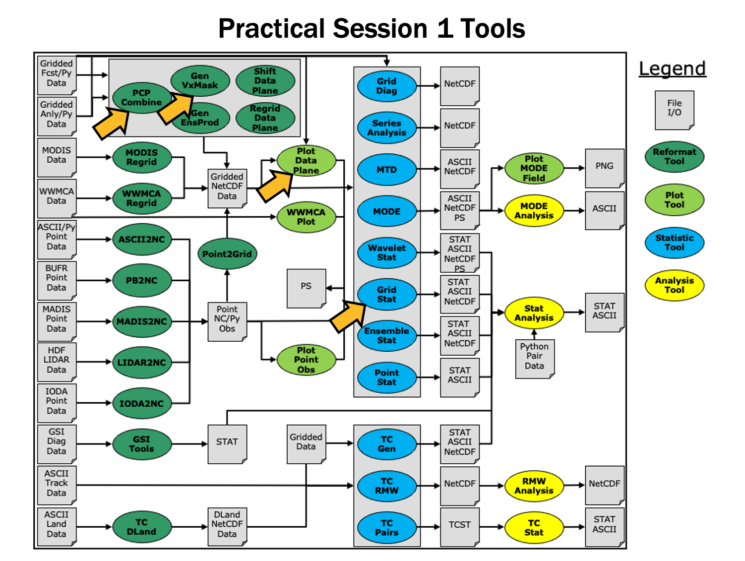
During this practical session, please work on the Session 1 exercises. Proceed through the tutorial exercises by following the navigation links at the bottom of each page.
Tutorial Format
Throughout this tutorial, code blocks in BOLD white text with a black background should be copied from your browser and pasted on the command line, e.g.:
Tutorial Tips
Note: Instructions in this tutorial use vi to open and edit files. If you prefer to use a different file editor, feel free to substitute it whenever you see vi.
Note: Instructions in this tutorial use okular to view pdf, ps, and png files. If you prefer to use a different file viewer, feel free to substitute it whenever you see okular.
Note: If you are running the tutorial inside Docker, you will not have access to the visualization tools described in this tutorial (such as okular, ncview, etc.) inside the Docker container. To run these commands, you will have to mount the output directory inside Docker to your local computer file system and run these tools from there.
MET Tool: PCP-Combine
MET Tool: PCP-Combine
We now shift to a discussion of the MET PCP-Combine tool and will practice running it directly on the command line.
PCP-Combine Functionality
The PCP-Combine tool is used (if needed) to add, subtract, sum or derive accumulated field values, most commonly precipitation, from several gridded data files into a single NetCDF file containing the desired accumulation period. Its NetCDF output may be used as input to the MET statistics tools. PCP-Combine may be configured to combine any gridded data field you'd like. However, all gridded data files being combined must have already been placed on a common grid. The copygb utility is recommended for re-gridding GRIB files. In addition, the PCP-Combine tool will only sum model files with the same initialization time unless it is configured to ignore the initialization time.
PCP-Combine Usage
View the usage statement for PCP-Combine by simply typing the following:
| Usage: pcp_combine | ||
| [[-sum] sum_args] | [-add input_files] | [-subtract input_files] | [-derive stat_list input_files] (Note: "|" means "or") |
||
| [-sum] sum_args | Data from multiple files containing the same accumulation interval should be summed up using the arguments provided. | |
| -add input_files | Data from one or more files should be added together where the accumulation interval is specified separately for each input file. | |
| -subtract input_files | Data from exactly two files should be subtracted. | |
| -derive stat_list input_files | The comma-separated list of statistics in "stat_list" (sum, min, max, range, mean, stdev, vld_count) should be derived using data from one or more files. | |
| out_file | Output NetCDF file to be written. | |
| [-field string] | Overrides the default use of accumulated precipitation (optional). | |
| [-name list] | Overrides the default NetCDF variable name(s) to be written (optional). | |
| [-vld_thresh n] | Overrides the default required ratio of valid data (1) (optional). | |
| [-log file] | Outputs log messages to the specified file | |
| [-v level] | Level of logging | |
| [-compress level] | NetCDF file compression |
Use the -sum, -add, -subtract, or -derive command line option to indicate the operation to be performed. Each operation has its own set of required arguments.
Run Sum Command
Run Sum Command
Since PCP-Combine performs a simple operation and reformatting step, no configuration file is needed.
- Start by making an output directory for PCP-Combine and changing directories:
cd ${METPLUS_TUTORIAL_DIR}/output/met_output/pcp_combine
- Now let's run PCP-Combine twice using some sample data that's included with the MET tarball:
-sum 20050807_000000 3 20050807_120000 12 \
sample_fcst_12L_2005080712V_12A.nc \
-pcpdir ${METPLUS_DATA}/met_test/data/sample_fcst/2005080700
pcp_combine \
-sum 00000000_000000 1 20050807_120000 12 \
sample_obs_12L_2005080712V_12A.nc \
-pcpdir ${METPLUS_DATA}/met_test/data/sample_obs/ST2ml
The "\" symbols in the commands above are used for ease of reading. They are line continuation markers enabling us to spread a long command line across multiple lines. They should be followed immediately by "Enter". You may copy and paste the command line OR type in the entire line with or without the "\".
Both commands run the sum command which searches the contents of the -pcpdir directory for the data required to create the requested accmululation interval.
In the first command, PCP-Combine summed up 4 3-hourly accumulation forecast files into a single 12-hour accumulation forecast. In the second command, PCP-Combine summed up 12 1-hourly accumulation observation files into a single 12-hour accumulation observation. PCP-Combine performs these tasks very quickly.
We'll use these PCP-Combine output files as input for Grid-Stat. So make sure that these commands have run successfully!
Output
Output
When PCP-Combine is finished, you may view the output NetCDF files it wrote using the ncdump and ncview utilities. Run the following commands to view contents of the NetCDF files:
ncview sample_obs_12L_2005080712V_12A.nc &
ncdump -h sample_fcst_12L_2005080712V_12A.nc
ncdump -h sample_obs_12L_2005080712V_12A.nc
The ncview windows display plots of the precipitation data in these files. The output of ncdump indicates that the gridded fields are named APCP_12, the GRIB code abbreviation for accumulated precipitation. The accumulation interval is 12 hours for both the forecast (3-hourly * 4 files = 12 hours) and the observation (1-hourly * 12 files = 12 hours).
Note, if ncview is not found when you run it on your system, you may need to load it first. For example, on hera, you can use this command:
Plot-Data-Plane Tool
The Plot-Data-Plane tool can be run to visualize any gridded data that the MET tools can read. It is a very helpful utility for making sure that MET can read data from your file, orient it correctly, and plot it at the correct spot on the earth. When using new gridded data in MET, it's a great idea to run it through Plot-Data-Plane first:
sample_fcst_12L_2005080712V_12A.nc \
sample_fcst_12L_2005080712V_12A.ps \
'name="APCP_12"; level="(*,*)";'
gv sample_fcst_12L_2005080712V_12A.ps &
Ghostview (gv) can take a little while before it displays. If you don't have gv on your computer, try using display, or any tool that can visualize PostScript files, e.g.:
Another option is to create a PNG file from the PS file, also rotating it to appear the right way:
sample_fcst_12L_2005080712V_12A.png
Next try re-running the command list above, but add the convert(x)=x/25.4; function to the config string (Hint: after the level setting and ; but before the last closing tick) to change units from millimeters to inches. What happened to the values in the colorbar?
Now, try re-running again, but add the censor_thresh=lt1.0; censor_val=0.0; options to the config string to reset any data values less 1.0 to a value of 0.0. How has your plot changed?
The convert(x) and censor_thresh/censor_val options can be used in config strings and MET config files to transform your data in simple ways.
Add and Subtract Commands
Add and Subtract Commands
We have run examples of the PCP-Combine -sum command, but the tool also supports the -add, -subtract, and -derive commands. While the -sum command defines a directory to be searched, for -add, -subtract, and -derive we tell PCP-Combine exactly which files to read and what data to process. The following command adds together 3-hourly precipitation from 4 forecast files, just like we did in the previous step with the -sum command:
${METPLUS_DATA}/met_test/data/sample_fcst/2005080700/wrfprs_ruc13_03.tm00_G212 03 \
${METPLUS_DATA}/met_test/data/sample_fcst/2005080700/wrfprs_ruc13_06.tm00_G212 03 \
${METPLUS_DATA}/met_test/data/sample_fcst/2005080700/wrfprs_ruc13_09.tm00_G212 03 \
${METPLUS_DATA}/met_test/data/sample_fcst/2005080700/wrfprs_ruc13_12.tm00_G212 03 \
add_APCP_12.nc
By default, PCP-Combine looks for accumulated precipitation, and the 03 tells it to look for 3-hourly accumulations. However, that 03 string can be replaced with a configuration string describing the data to be processed, which doesn't have to be accumulated precipation. The configuration string should be enclosed in single quotes. Below, we add together the U and V components of 10-meter wind from the same input file. You would not typically want to do this, but this demonstrates the functionality. We also use the -name command line option to define a descriptive output NetCDF variable name:
${METPLUS_DATA}/met_test/data/sample_fcst/2005080700/wrfprs_ruc13_03.tm00_G212 'name="UGRD"; level="Z10";' \
${METPLUS_DATA}/met_test/data/sample_fcst/2005080700/wrfprs_ruc13_03.tm00_G212 'name="VGRD"; level="Z10";' \
add_WINDS.nc \
-name UGRD_PLUS_VGRD
While the -add command can be run on one or more input files, the -subtract command requires exactly two. Let's rerun the wind example from above but do a subtraction instead:
${METPLUS_DATA}/met_test/data/sample_fcst/2005080700/wrfprs_ruc13_03.tm00_G212 'name="UGRD"; level="Z10";' \
${METPLUS_DATA}/met_test/data/sample_fcst/2005080700/wrfprs_ruc13_03.tm00_G212 'name="VGRD"; level="Z10";' \
subtract_WINDS.nc \
-name UGRD_MINUS_VGRD
Now run Plot-Data-Plane to visualize this output. Use the -plot_range option to specify a the desired plotting range, the -title option to add a title, and the -color_table option to switch from the default color table to one that's good for positive and negative values:
subtract_WINDS.nc \
subtract_WINDS.ps \
'name="UGRD_MINUS_VGRD"; level="(*,*)";' \
-plot_range -15 15 \
-title "10-meter UGRD minus VGRD" \
-color_table ${MET_BUILD_BASE}/share/met/colortables/NCL_colortables/posneg_2.ctable
Now view the results:
Derive Command
Derive Command
While the PCP-Combine -add and -subtract commands compute exactly one output field of data, the -derive command can compute multiple output fields in a single run. This command reads data from one or more input files and derives the output fields requested on the command line (sum, min, max, range, mean, stdev, vld_count).
Run the following command to derive several summary metrics for both the 10-meter U and V wind components:
${METPLUS_DATA}/met_test/data/sample_fcst/2005080700/wrfprs_ruc13_*.tm00_G212 \
-field 'name="UGRD"; level="Z10";' \
-field 'name="VGRD"; level="Z10";' \
derive_min_max_mean_stdev_WINDS.nc
In the above example, we used a wildcard to list multiple input file names. And we used the -field command line option twice to specify two input fields. For each input field, PCP-Combine loops over the input files, derives the requested metrics, and writes them to the output NetCDF file. Run ncview to visualize this output:
This output file contains 8 variables: 2 input fields * 4 metrics. Note the output variable names the tool chose. You can still override those names using the -name command line argument, but you would have to specify a comma-separated list of 8 names, one for each output variable.
MET Tool: Plot-Data-Plane
MET Tool: Plot-Data-Plane
Whenever getting started with new gridded datasets in MET, users are strongly encouraged to first run the Plot-Data-Plane tool to visualize the data. Doing so confirms that MET can read the input file, extract the desired data, and geolocate and orient it correctly. It is particularly useful in testing the configuration string needed to extract the data from the input file.
Plot-Data-Plane Functionality
The Plot-Data-Plane tool reads a single 2-dimensional field of gridded data from the specified input file and writes a PostScript output file containing a spatial plot of the data. It plots the data using a configurable color table that is automatically rescaled to the range of values found by default. The ImageMagick convert utility is recommend for converting the PostScript output file to other image file formats, if needed.
Plot-Data-Plane Usage
| Usage: plot_data_plane | ||
| input_filename | Input file containing gridded data to be be plotted | |
| output_filename | Output PostScript file to be written | |
| field_string | String defining the data to be plotted | |
| [-color_table name] | Overrides the default color table (optional) | |
| [-plot_range min max] | Specifies the range of data to be plotted (optional) | |
| [-title string] | Specifies the plot title string (optional) | |
| [-log file] | Outputs log messages to the specified file | |
| [-v level] | Level of logging |
The Field String
The Field String
Defining the field string
As you'll see throughout these exercises, the behavior of the MET and METplus tools is controlled using ASCII configuration files, and you will learn more about those options in the coming sessions. The field_string command line argument is actually processed as a miniature configuration file. In fact, that string is written to a temporary file which is then read by MET's configuration file library code.
In general, the name and level entries are required to extract a gridded field of data from a supported input file format. The conventions for specifying them vary based on the input file type:
- For GRIB1 or GRIB2 inputs, set name as the abbreviation for the desired variable or data type that appears in the GRIB tables and set level to a single letter (A, Z, P, L, or R) to define the level type followed by a number to define the level value. For example 'name = "TMP"; level = "P500";' extracts 500 millibar temperature from a GRIB file.
- For NetCDF inputs, set name as the NetCDF variable name and level to define how to extract a 2-dimensional slice of gridded data from that variable. For example, 'name = "temperature"; level = "(0,1,*,*)";' extracts a 2-dimensional field of data from the last two dimensions of a NetCDF temperature variable using the first two indicies as constant values.
- For Python embedding, set name as the python script to be run along with any arguments for that script and do not set level. For example, 'name = "read_my_data.py input.txt";' runs a python script to read data from the specified input file.
Note that all field strings should be enclosed in single quotes, as shown above, so that they are processed on the command line as a single string which may contain embedded whitespace.
Examples for each of these input types are provided in the coming exercises. More details about setting the field string can be found in the Configuration File Overview section of the MET User's Guide. For example, if a field string matches multiple records in an input GRIB file, additional filtering criteria may be specified to further refine them. Additional options exist to explicitly specify the input file_type, define a function to convert the data, or define an operation to censor the data. Each configuration entry should be terminated with a semi-colon (;).
Since the field_string is processed using a temporary file, any syntax errors will produce a parsing error log message similar to the following:
ERROR : yyerror() -> syntax error in file "/tmp/met_config_61354_1"
ERROR :
Error messages like this typically mean there is a problem in a configuration string or configuration file being read by MET.
Plot GRIB Data
Plot GRIB Data
Plot GRIB Data
Start by creating a directory for our Plot-Data-Plane output:
Next, run Plot-Data-Plane to plot 2-meter temperature from a GRIB1 input file:
${METPLUS_DATA}/met_test/data/sample_fcst/2005080700/wrfprs_ruc13_12.tm00_G212 \
${METPLUS_TUTORIAL_DIR}/output/met_output/plot_data_plane/wrfprs_TMP_2m.ps \
'name = "TMP"; level = "Z2";'
The default verbosity level of 2 only prints log messages about input and output files.
DEBUG 1: Creating postscript file: {...}/wrfprs_TMP_2m.ps
Next, re-run at verbosity level 4 to see more detailed log message about the grid being read, timing information, and the range of the data values:
${METPLUS_DATA}/met_test/data/sample_fcst/2005080700/wrfprs_ruc13_12.tm00_G212 \
${METPLUS_TUTORIAL_DIR}/output/met_output/plot_data_plane/wrfprs_TMP_2m.ps \
'name = "TMP"; level = "Z2";' -v 4
It is a great idea to inspect the log messages to sanity check the metadata. Without needing to understand all the details, does the grid definition look reasonable? Are the range of values reasonable for this variable type? Are the timestamps of the data consistent with the input file name?
Next, open the PostScript output file. On some machines, the ghostview utility (or common gv alias) can display PostScript files. On other, the display command works well. On Macs, simply run open. The example below uses gv which is available in the METplus AMI:
Optionally, if the convert utility is in your path, it can be run to change the image file format. Indicate the desired output file format by specifying the suffix (.png shown below).
${METPLUS_TUTORIAL_DIR}/output/met_output/plot_data_plane/wrfprs_TMP_2m.ps \
${METPLUS_TUTORIAL_DIR}/output/met_output/plot_data_plane/wrfprs_TMP_2m.png
The plot is created using the default color table (met_default.ctable) and is scaled to the range of valid data (275 to 305). By default, no title is provided and the input file is listed as a sub-title. Does the pattern of the data look reasonable? Does it correspond well to the background map data?
If the plot of the data and the metadata listed in the log messages look reasonable, you can be confident that MET is reading your data well. In addition, the field_string you used to retrieve this data can be used in the configuration strings and configuration files for other MET tools.
While this Plot-Data-Plane validation step is not necessary for every input file, it is very useful when getting started with new input data sources.
Plot NetCDF Data
Plot NetCDF Data
Plot NetCDF Data
The NetCDF file format is very flexible and enables the creation of self-describing data files. However, that flexibility makes it impossible to write general purpose software to interpret all NetCDF files. For that reason, MET supports a few types of NetCDF file formats, but does not support all NetCDF files, in general. It can ingest NetCDF files that follow the Climate-Forecast Convention, are created by the WRF-Interp utility, or are created by other MET tools. Additional details can be found in the MET Data I/O chapter of the MET User's Guide.
As described in The Field String, set name to the name of the desired NetCDF variable and level to define how to index into the dimensions of that variable. In the NetCDF level strings, use *,* to indicate the two gridded dimensions. For other, non-gridded dimensions, pick a 0-based integer to specify the value to be used for that dimension. For the time dimension, if present, selecting a 0-based integer does work, however you can also specify a time string in YYYYMMDD[_HH[MMSS]] format. The square braces indicate optional elements of the format. So 19770807, 19770807_12, and 19770807_120000 are all valid time strings. It is often easier to specify a time string directly rather than finding the integer index corresponding to that time string.
Run Plot-Data-Plane to plot quantitative precipitation estimate (QPE) data from a CF-compliant NetCDF file. First run ncdump -h to take a look at the header:
${METPLUS_DATA}/model_applications/precipitation/QPE_Data/20170510/qpe_2017051005.nc
Note the following from the header:
time = 1 ;
y = 689 ;
x = 1073 ;
...
float P06M_NONE(time, y, x) ;
...
// global attributes:
:Conventions = "CF-1.0" ;
The variable P06M_NONE has 3 dimensions, but the time dimension only has length 1. Therefore, setting level = "(0,*,*)"; should do the trick. Also note that the global Conventions attribute identifies this file as being CF-compliant. Let's plot it, this time adding a title:
${METPLUS_DATA}/model_applications/precipitation/QPE_Data/20170510/qpe_2017051005.nc \
${METPLUS_TUTORIAL_DIR}/output/met_output/plot_data_plane/qpe_2017051005.ps \
'name = "P06M_NONE"; level = "(0,*,*)";' -title "Precipitation Forecast" -v 4
Running at verbosity level 4, we see the range of values:
DEBUG 4: plane min: 0
DEBUG 4: plane max: 101.086
If needed, run convert to reformat:
${METPLUS_TUTORIAL_DIR}/output/met_output/plot_data_plane/qpe_2017051005.ps \
${METPLUS_TUTORIAL_DIR}/output/met_output/plot_data_plane/qpe_2017051005.png
The next example extracts a specific time string from a precipitation analysis dataset:
${METPLUS_DATA}/model_applications/precipitation/StageIV/2017050912_st4.nc
Note the following from the header:
time = 4 ;
y = 428 ;
x = 614 ;
time1 = 1 ;
variables:
float P06M_NONE(time, y, x) ;
Let's request a specific time string, specify a title, and use the same plotting range as above, rather than defaulting to the range of input data values.
${METPLUS_DATA}/model_applications/precipitation/StageIV/2017050912_st4.nc \
${METPLUS_TUTORIAL_DIR}/output/met_output/plot_data_plane/2017050912_st4.ps \
'name = "P06M_NONE"; level = "(20170510_06,*,*)";' \
-plot_range 0 101.086 -title "Precipitation Analysis"
If running Plot-Data-Plane for multiple output times or data sources, consider using the -plot_range option to make their color scales comparable.
Lastly, let's plot output a NetCDF mask file that was created by an earlier version of MET's Gen-Vx-Mask tool.
We will plot the NCEP_Region_ID variable with only 2 dimensions:
Let's specify a different color table rather than using the default one.
${METPLUS_DATA}/met_test/data/poly/NCEP_masks/NCEP_Regions.nc \
${METPLUS_TUTORIAL_DIR}/output/met_output/plot_data_plane/NCEP_Regions.ps \
'name = "NCEP_Region_ID"; level = "(*,*)";' \
-color_table $MET_BUILD_BASE/share/met/colortables/NCL_colortables/rainbow.ctable
Python Embedding
Python Embedding
Python Embedding
While the MET tools can read data from a few input gridded data file types, its ability to read data in memory from python greatly enhances its utility. Support for python embedding is optional, and must be enabled at compilation time as described in Appendix F of the MET User's Guide. MET supports three types of python embedding:
- Reading a field of gridded data values.
- Passing a list of point observations.
- Passing a list of matched forecast/observation pair values.
On this page, we'll demonstrate only the first type, reading a field of gridded data values. When getting started with a new dataset via python, validating the logic by running Plot-Data-Plane is crucial. When MET reads data from flat files, important information, like the location and orientation of the data, is defined in the metadata. That is not the case for python embedding, and the responsibility for confirming those details falls to the user. So while python embedding provide extra flexibility, it also requires additional diligence.
Let's run the simplest of examples using sample data included with the MET release. The first step is to confirm that python script runs by itself, outside of MET.
${METPLUS_DATA}/met_test/data/python/fcst.txt Forecast
This sample read_ascii_numpy.py script reads data from the input fcst.txt ASCII file and gives it a name, Forecast. Always run new python scripts on the command line first to confirm there aren't any syntax errors in the script itself. The required conventions for the python script are details in the Python Embedding for 2D Data section of the MET User's Guide.
Next, let's run Plot-Data-Plane using this python script to define the input data. As described in The Field String, this is done with the name configuration string and the level string does not apply.
PYTHON_NUMPY \
${METPLUS_TUTORIAL_DIR}/output/met_output/plot_data_plane/python_fcst.ps \
'name = "${METPLUS_DATA}/met_test/scripts/python/read_ascii_numpy.py ${METPLUS_DATA}/met_test/data/python/fcst.txt Forecast";'
Since there is no input_filename to be specified as the first required argument for Plot-Data-Plane, we provide the constant string PYTHON_NUMPY in that spot. This triggers Plot-Data-Plane to interpret the field string as a python embedding script to be run. Specifying PYTHON_XARRAY also works but requires slightly different conventions in the python embedding script.
When MET is compiled, it links to python libraries that it uses to instantiate a python interpreter at runtime. That compile time instance does have a few required packages, but will likely not include all packages that every user may want to load. You may find that your python script runs fine on the command line, but Plot-Data-Plane's call to python can't load a requested module. In that case, set the ${MET_PYTHON_EXE} environment variable to tell MET which instance of python you'd like to run.
The following command just uses that version of python that is already present in your path:
Rerunning the command from above should produce the same result, but if you look closely at the log messages, you'll see that your custom python version writes a temporary file, and MET's compile time python version reads data from it.
PYTHON_NUMPY \
${METPLUS_TUTORIAL_DIR}/output/met_output/plot_data_plane/python_fcst.ps \
'name = "${METPLUS_DATA}/met_test/scripts/python/read_ascii_numpy.py ${METPLUS_DATA}/met_test/data/python/fcst.txt Forecast";'
You can find several python embedding examples on the Sample Analysis Scripts page of the MET website. Each example includes both a python script and sample input data file. Please also see METplus Python Embedding use case examples.
MET Tool: Gen-Vx-Mask
MET Tool: Gen-Vx-Mask
Gen-Vx-Mask Functionality
The Gen-Vx-Mask tool may be run to speed up the execution time of the other MET tools. Gen-Vx-Mask defines a bitmap masking region for your domain. It takes as input a gridded data file defining your domain and a second argument to define the area of interest (varies by masking type). It writes out a NetCDF file containing a bitmap for that masking region. You can run Gen-Vx-Mask iteratively, passing its output back in as input, to define more complex masking regions.
You can then use the output of Gen-Vx-Mask to define masking regions in the MET statistics tools. While those tools can read ASCII lat/lon polyline files directly, they are able to process the output of Gen-Vx-Mask much more quickly than the original polyline. The idea is to define your masking region once for your domain with Gen-Vx-Mask and apply the output many times in the MET statistics tools.
Gen-Vx-Mask Usage
View the usage statement for Gen-Vx-Mask by simply typing the following:
| Usage: gen_vx_mask | ||
| input_file | Gridded data file defining the domain | |
| mask_file | Defines the masking region and varies by -type | |
| out_file | Output NetCDF mask file to be written | |
| -type string | Masking type: poly, poly_xy, box, circle, track, grid, data, solar_alt, solar_azi, lat, lon, shape | |
| [-input_field string] | Define field from input_file for grid point initialization values, rather than 0. | |
| [-mask_field string] | Define field from mask_file for data masking. | |
| [-complement, -union, -intersection, -symdiff] | Set logic for combining input_field initialization values with the current mask values. | |
| [-thresh string] | Define threshold for circle, track, data, solar_alt, solar_azi, lat, and lon masking types. | |
| [-height n, -width n] | Define dimensions for box masking. | |
| [-shapeno n] | Define the index of the shape for shapefile masking. | |
| [-value n] | Output mask value to be written, rather than 1. | |
| [-name str] | Specifies the name to be used for the mask. | |
| [-log file] | Outputs log messages to the specified file | |
| [-v level] | Level of logging | |
| [-compress level] | NetCDF compression level |
At a minimum, the input data_file, the input mask_poly polyline file, the output netcdf_file, and the type must be passed on the command line.
Run Poly Type
Run Poly Type
Start by making an output directory for Gen-Vx-Mask and changing directories:
cd ${METPLUS_TUTORIAL_DIR}/output/met_output/gen_vx_mask
Since Gen-Vx-Mask performs a simple masking step, no configuration file is needed.
We'll run the Gen-Vx-Mask tool to apply a polyline for the CONUS (Contiguous United States) to our model domain. Run Gen-Vx-Mask on the command line using the following command:
${METPLUS_DATA}/met_test/data/sample_obs/ST2ml/ST2ml2005080712.Grb_G212 \
${MET_BUILD_BASE}/share/met/poly/CONUS.poly \
CONUS_mask.nc \
-type poly -v 2
Re-run using verbosity level 3 and look closely at the log messages. How many grid points were included in this mask?
Gen-Vx-Mask should run very quickly since the grid is coarse (185x129 points) and there are 243 lat/lon points in the CONUS polyline. The more you increase the grid resolution and number of polyline points, the longer it will take to run. View the NetCDF bitmap file generated by executing the following command:
Notice that the bitmap has a value of 1 inside the CONUS polyline and 0 everywhere else. We'll use the CONUS mask we just defined in the next step.
You could try running plot_data_plane to create a PostScript image of this masking region. Can you remember how?
Notice that there are several ways that gen_vx_mask can be run to define regions of interest, some of which will be demonstrated over the next few pages.
Run Lat/Lon and Grid Types
Run Lat/Lon and Grid Types
Using a pre-defined NCEP grid from the NCEP ON388 Grid Identification Table, we'll create a latitude band, using the "lat" masking type, for the tropics region. Run Gen-Vx-Mask on the command line using the following command:
G004 \
G004 \
${METPLUS_TUTORIAL_DIR}/output/met_output/gen_vx_mask/G004_Tropics.nc \
-type lat -thresh 'ge-30 && le30'
Most of the grids defined in ON388 Table B can be referenced in MET as "GNNN" where NNN is the 3-digit grid number. Run "ncdump -h" on the output file and notice that the mask variable is named "lat_mask":
lat_mask:long_name = "lat_mask masking region" ;
lat_mask:_FillValue = -9999.f ;
lat_mask:mask_type = "lat>=-30&&<=30" ;
Use the "-name" command line option, as shown below, to override this default.
To compute the intersection or union of two masks, use the output from the first run as input to the second. Run Gen-Vx-Mask on the command line using the following command, which uses the "lon" masking type:
${METPLUS_TUTORIAL_DIR}/output/met_output/gen_vx_mask/G004_Tropics.nc \
${METPLUS_TUTORIAL_DIR}/output/met_output/gen_vx_mask/G004_Tropics.nc \
${METPLUS_TUTORIAL_DIR}/output/met_output/gen_vx_mask/G004_EastPac.nc \
-type lon -thresh 'le-70 && ge-130' -intersection -name EastPac
Compare this intersection output to the union of the two masks, computed below:
${METPLUS_TUTORIAL_DIR}/output/met_output/gen_vx_mask/G004_Tropics.nc \ ${METPLUS_TUTORIAL_DIR}/output/met_output/gen_vx_mask/G004_Tropics.nc \
${METPLUS_TUTORIAL_DIR}/output/met_output/gen_vx_mask/G004_EastPac.nc \
-type lon -thresh 'le-70 && ge-130' -union
Now we'll use the "grid" masking type to select a subgrid from a larger grid. Run Gen-Vx-Mask on the command line using the following command:
G004 \
${METPLUS_DATA}/met_test/data/sample_obs/ST2ml/ST2ml2005080712.Grb_G212 \
${METPLUS_TUTORIAL_DIR}/output/met_output/gen_vx_mask/G004_SUBGRID.nc \
-type grid
On the next page, we'll demonstrate using the "data" and "solar_alt" masking types.
Run Data and Solar Types
Run Data and Solar Types
On this page, we provide examples for land/sea mask and also a solar altitude to show where it is daytime on a global grid.
Run Gen-Vx-Mask on the command line using the following command:
${METPLUS_DATA}/model_applications/medium_range/grid_to_obs/gfs/pgbf00.gfs.2017060100 \
${METPLUS_DATA}/model_applications/medium_range/grid_to_obs/gfs/pgbf00.gfs.2017060100 \
${METPLUS_TUTORIAL_DIR}/output/met_output/gen_vx_mask/GFS_LAND.nc \
-type data -mask_field 'name="LAND"; level="L0";' -thresh eq1 -name LAND
A corresponding water mask could be created using two different methods. One way is to simply rerun the land mask command above using the -complement option:
${METPLUS_DATA}/model_applications/medium_range/grid_to_obs/gfs/pgbf00.gfs.2017060100 \
${METPLUS_DATA}/model_applications/medium_range/grid_to_obs/gfs/pgbf00.gfs.2017060100 \
${METPLUS_TUTORIAL_DIR}/output/met_output/gen_vx_mask/GFS_LAND_COMP.nc \
-type data -mask_field 'name="LAND"; level="L0";' -thresh eq1 -name LAND_COMP -complement
Another way is to specify a different threshold (eq1 instead of eq0) rather than taking the complement:
${METPLUS_DATA}/model_applications/medium_range/grid_to_obs/gfs/pgbf00.gfs.2017060100 \
${METPLUS_DATA}/model_applications/medium_range/grid_to_obs/gfs/pgbf00.gfs.2017060100 \
${METPLUS_TUTORIAL_DIR}/output/met_output/gen_vx_mask/GFS_WATER.nc \
-type data -mask_field 'name="LAND"; level="L0";' -thresh eq0 -name WATER
Now we'll run Gen-Vx-Mask to show where it’s daytime on a global grid:
G004 \
20170601_183000 \
${METPLUS_TUTORIAL_DIR}/output/met_output/gen_vx_mask/SOLAR_DAY.nc \
-type solar_alt -thresh ge0 -name DAY
Next, combine the LAND output from the previous run with the solar altitude mask for daytime:
${METPLUS_TUTORIAL_DIR}/output/met_output/gen_vx_mask/GFS_LAND.nc \
20170601_183000 \
${METPLUS_TUTORIAL_DIR}/output/met_output/gen_vx_mask/DAYLIGHT_LAND.nc \
-type solar_alt -thresh ge0 -name DAYLIGHT_LAND -intersection
This creates a mask for grid points on land experiencing daylight at 18:30 UTC on 20170601.
On the next page, we'll demonstrate using the "track" and "circle" masking types.
Run Track and Circle Types
Run Track and Circle Types
On this page, we provide examples for using the "track" masking type using BEST track hurricane data and "circle" masking type.
Start by extracting the lat/lon locations for Hurricane Dorian:
Inspect the dorian.poly file that begins with "DORIAN" and has the lat/lon storm locations on subsequent lines.
Compute a mask for all grid points within 200 km of the Hurricane Dorian track. Run Gen-Vx-Mask using the following command:
G003 \
${METPLUS_TUTORIAL_DIR}/output/met_output/gen_vx_mask/dorian.poly \
${METPLUS_TUTORIAL_DIR}/output/met_output/gen_vx_mask/Dorian_Track.nc \
-type track -name Dorain_Track -thresh le200
Extract the first track point for Dorian and use the circle masking option to select all grid points within 500 km:
Run Gen-Vx-Mask on the command line using the following command:
G003 \
${METPLUS_TUTORIAL_DIR}/output/met_output/gen_vx_mask/dorian_first.poly \
${METPLUS_TUTORIAL_DIR}/output/met_output/gen_vx_mask/Dorian_Origin.nc \
-type circle -name Dorain_Track -thresh le500
The "circle" mask type draws a circle around each of the lat/lon points in the input poly file. The "circle" option may be useful when verifying within a certain radius of known radar locations. If you rerun without the "-thresh" command line option, Gen-Vx-Mask still runs but prints a warning message:
Can you figure out what this output file now contains? Run ncview or plot_data_plane to visualize it.
Gen-Vx-Mask also supports the "box", "solar_azi", and "shape" masking types, not covered in these exercises. Interested users can download Natural Earth shapefiles and run Gen-Vx-Mask using the "-type shape" option.
Next, we'll take a look at using the "shape" masking type with Gen-Vx-Mask.
Run Shape Type
Run Shape Type
We will demonstrate the Gen-Vx-Mask "shape" masking type using freely available shapefiles from Natural Earth. While multiple resolutions are provided, we'll use the coarsest version for this example since it's the smallest in size.
Download the Natural Earth administrative shapefiles for countries boundaries.
mkdir ne_shapefiles; cd ne_shapefiles
wget https://naciscdn.org/naturalearth/110m/cultural/ne_110m_admin_0_countries.zip
unzip ne_110m_admin_0_countries.zip
Run gen_vx_mask to define the mask for the USA (index 4).
Re-run to compute the union with Canada (index 3).
Re-run to add Mexico (index 27).
The result is good but not perfect. There are a few missing grid points along the boundary. But this demonstrates how the tool works. Consider re-running all three commands again, but this time use the "-value" command line option to define the mask value to be written. Just make "-value" match the "-shapeno" option (.e.g. -value 4 for USA, -value 3 for Canada, and -value 27, for Mexico). What impact does that have on the result?
Next, we'll take a look at the functionality that Grid-Stat offers.
MET Tool: Grid-Stat
MET Tool: Grid-Stat
Grid-Stat Functionality
The Grid-Stat tool provides verification statistics for a matched forecast and observation grid. If the forecast and observation grids do not match, the regrid section of the configuration file controls how the data can be interpolated to a common grid. All of the forecast gridpoints in each spatial verification region of interest are matched to observation gridpoints. The matched gridpoints within each verification region are used to compute the verification statistics.
The output statistics generated by Grid-Stat include continuous partial sums and statistics, vector partial sums and statistics, categorical tables and statistics, probabilistic tables and statistics, neighborhood statistics, and gradient statistics. The computation and output of these various statistics types is controlled by the output_flag in the configuration file.
Grid-Stat Usage
View the usage statement for Grid-Stat by simply typing the following:
| Usage: grid_stat | ||
| fcst_file | Input gridded forecast file containing the field(s) to be verified. | |
| obs_file | Input gridded observation file containing the verifying field(s). | |
| config_file | GridStatConfig file containing the desired configuration settings. | |
| [-outdir path] | Overrides the default output directory (optional). | |
| [-log file] | Outputs log messages to the specified file (optional). | |
| [-v level] | Level of logging (optional). | |
| [-compress level] | NetCDF compression level (optional). |
The forecast and observation fields must be on the same grid for verification. You can use copygb to regrid GRIB1 files, wgrib2 to regrid GRIB2 files, or the automated regridding within the regrid section of the MET config files.
At a minimum, the input gridded fcst_file, the input gridded obs_file, and the configuration config_file must be passed in on the command line.
Configure
Configure
Start by making an output directory for Grid-Stat and changing directories:
cd ${METPLUS_TUTORIAL_DIR}/output/met_output/grid_stat
The behavior of Grid-Stat is controlled by the contents of the configuration file passed to it on the command line. The default Grid-Stat configuration file may be found in the data/config/GridStatConfig_default file. Prior to modifying the configuration file, users are advised to make a copy of the default:
Open up the GridStatConfig_tutorial file for editing with your preferred text editor.
The configurable items for Grid-Stat are used to specify how the verification is to be performed. The configurable items include specifications for the following:
- The forecast fields to be verified at the specified vertical level or accumulation interval
- The threshold values to be applied
- The areas over which to aggregate statistics - as predefined grids, configurable lat/lon polylines, or gridded data fields
- The confidence interval methods to be used
- The smoothing methods to be applied (as opposed to interpolation methods)
- The types of verification methods to be used
You may find a complete description of the configurable items in the grid_stat configuration file section of the MET User's Guide. Please take some time to review them.
For this tutorial, we'll configure Grid-Stat to verify the 12-hour accumulated precipitation output of PCP-Combine. We'll be using Grid-Stat to verify a single field using NetCDF input for both the forecast and observation files. However, Grid-Stat may in general be used to verify an arbitrary number of fields. Edit the GridStatConfig_tutorial file as follows:
- Set:
fcst = {
field = [
{
name = "APCP_12";
level = [ "(*,*)" ];
cat_thresh = [ >0.0, >=5.0, >=10.0 ];
}
];
}
obs = fcst;To verify the field of precipitation accumulated over 12 hours using the 3 thresholds specified.
- Set:
mask = {
grid = [];
poly = [ "../gen_vx_mask/CONUS_mask.nc",
"MET_BASE/poly/NWC.poly",
"MET_BASE/poly/SWC.poly",
"MET_BASE/poly/GRB.poly",
"MET_BASE/poly/SWD.poly",
"MET_BASE/poly/NMT.poly",
"MET_BASE/poly/SMT.poly",
"MET_BASE/poly/NPL.poly",
"MET_BASE/poly/SPL.poly",
"MET_BASE/poly/MDW.poly",
"MET_BASE/poly/LMV.poly",
"MET_BASE/poly/GAC.poly",
"MET_BASE/poly/APL.poly",
"MET_BASE/poly/NEC.poly",
"MET_BASE/poly/SEC.poly" ];
}To accumulate statistics over the Continental United States (CONUS) and the 14 NCEP verification regions in the United States defined by the polylines specified. To see a plot of these regions, execute the following command:
gv ${MET_BUILD_BASE}/share/met/poly/ncep_vx_regions.pdf & - In the boot dictionary, set:
n_rep = 500;To turn on the computation of bootstrap confidence intervals using 500 replicates.
- In the nbrhd dictionary, set:
width = [ 3, 5 ];
cov_thresh = [ >=0.5, >=0.75 ];To define two neighborhood sizes and two fractional coverage field thresholds.
- Set:
output_flag = {
fho = NONE;
ctc = BOTH;
cts = BOTH;
mctc = NONE;
mcts = NONE;
cnt = BOTH;
sl1l2 = BOTH;
sal1l2 = NONE;
vl1l2 = NONE;
val1l2 = NONE;
vcnt = NONE;
pct = NONE;
pstd = NONE;
pjc = NONE;
prc = NONE;
eclv = NONE;
nbrctc = BOTH;
nbrcts = BOTH;
nbrcnt = BOTH;
grad = BOTH;
dmap = NONE;
seeps = NONE;
}To compute contingency table counts (CTC), contingency table statistics (CTS), continuous statistics (CNT), scalar partial sums (SL1L2), neighborhood contingency table counts (NBRCTC), neighborhood contingency table statistics (NBRCTS), and neighborhood continuous statistics (NBRCNT).
Run
Run
Next, run Grid-Stat on the command line using the following command:
${METPLUS_TUTORIAL_DIR}/output/met_output/pcp_combine/sample_fcst_12L_2005080712V_12A.nc \
${METPLUS_TUTORIAL_DIR}/output/met_output/pcp_combine/sample_obs_12L_2005080712V_12A.nc \
${METPLUS_TUTORIAL_DIR}/output/met_output/grid_stat/GridStatConfig_tutorial \
-outdir ${METPLUS_TUTORIAL_DIR}/output/met_output/grid_stat \
-v 2
Grid-Stat is now performing the verification tasks we requested in the configuration file. It should take a minute or two to run. The status messages written to the screen indicate progress.
In this example, Grid-Stat performs several verification tasks in evaluating the 12-hour accumulated precipiation field:
- For continuous statistics and partial sums (CNT and SL1L2), 15 output lines each:
(1 field * 15 masking regions) - For contingency table counts and statistics (CTC and CTS), 45 output lines each:
(1 field * 3 raw thresholds * 15 masking regions) - For neighborhood methods (NBRCNT, NBRCTC, and NBRCTS), 90 output lines each:
(1 field * 3 raw thresholds * 2 neighborhood sizes * 15 masking regions)
To greatly increase the runtime performance of Grid-Stat, you could disable the computation of bootstrap confidence intervals in the configuration file. Edit the GridStatConfig_tutorial file as follows:
- In the boot dictionary, set:
n_rep = 0;To disable the computation of bootstrap confidence intervals.
Now, try rerunning the Grid-Stat command listed above and notice how much faster it runs. While bootstrap confidence intervals are nice to have, they take a long time to compute, especially for gridded data.
Output
Output
The output of Grid-Stat is one or more ASCII files containing statistics summarizing the verification performed and a NetCDF file containing difference fields. In this example, the output is written to the current directory, as we requested on the command line. It should now contain 10 Grid-Stat output files beginning with the grid_stat_ prefix, one each for the CTC, CTS, CNT, SL1L2, GRAD, NBRCTC, NBRCTS, and NBRCNT ASCII files, a STAT file, and a NetCDF matched pairs file.
The format of the CTC, CTS, CNT, and SL1L2 ASCII files will be covered for the Point-Stat tool. The neighborhood method and gradient output are unique to the Grid-Stat tool.
- Rather than comparing forecast/observation values at individual grid points, the neighborhood method compares areas of forecast values to areas of observation values. At each grid box, a fractional coverage value is computed for each field as the number of grid points within the neighborhood (centered on the current grid point) that exceed the specified raw threshold value. The forecast/observation fractional coverage values are then compared rather than the raw values themselves.
- Gradient statistics are computed on the forecast and observation gradients in the X and Y directions.
Since the lines of data in these ASCII files are so long, we strongly recommend configuring your text editor to NOT use dynamic word wrapping. The files will be much easier to read that way.
Execute the following command to view the NetCDF output of Grid-Stat:
Click through the 2d vars variable names in the ncview window to see plots of the forecast, observation, and difference fields for each masking region. If you see a warning message about the min/max values being zero, just click OK.
Now dump the NetCDF header:
View the NetCDF header to see how the variable names are defined.
Notice how *MANY* variables there are, separate output for each of the masking regions defined. Try editing the config file again by setting apply_mask = FALSE; and gradient = TRUE; in the nc_pairs_flag dictionary. Re-run Grid-Stat and inspect the output NetCDF file. What affect did these changes have?
METplus Motivation
METplus Motivation
We have now successfully run the PCP-Combine and Grid-Stat tools to verify 12-hourly accumulated preciptation for a single output time. We did the following steps:
- Identified our forecast and observation datasets.
- Constructed PCP-Combine commands to put them into a common accumulation interval.
- Configured and ran Grid-Stat to compute our desired verification statistics.
Now that we've defined the logic for a single run, the next step would be writing a script to automate these steps for many model initializations and forecast lead times. Rather than every MET user rewriting the same type of scripts, use METplus to automate these steps in a use case!
METplus Use Case: GridStat
METplus Use Case: GridStat
The GridStat use case utilizes the MET Grid-Stat tool.
Optional: Refer to the MET Users Guide for a description of the MET tools used in this use case.
Optional: Refer to the METplus Config Glossary section of the METplus Users Guide for a reference to METplus variables used in this use case.
Change to the ${METPLUS_TUTORIAL_DIR}
- Review the use case configuration file: GridStat.conf
Open the file and look at all of the configuration variables that are defined. This use-case shows a simple example of running Grid-Stat on 3-hour accumulated precipitation forecasts from WRF to Stage II quantitative precipitation estimates.
In METplus configuration files, the forecast and observation variables are referred to individually, including reference to both the NAMES and LEVELS.
FCST_VAR1_NAME = APCP
FCST_VAR1_LEVELS = A03
OBS_VAR1_NAME = APCP_03
OBS_VAR1_LEVELS = "(*,*)"
These relate to the following fields in the MET configuration file
field = [
{
name = "APCP";
level = [ "A03" ];
}
];
}
obs = {
field = [
{
name = "APCP_03";
level = [ "(*,*)" ];
}
];
}
Paths in GridStat.conf may reference other config options defined in a different configuration file. For example:
where INPUT_BASE which is set in the tutorial.conf configuration file. METplus config variables can reference other config variables even if they are defined in a config file that is read afterwards.
- Run the use case:
${METPLUS_BUILD_BASE}/parm/use_cases/met_tool_wrapper/GridStat/GridStat.conf \
${METPLUS_TUTORIAL_DIR}/tutorial.conf \
config.OUTPUT_BASE=${METPLUS_TUTORIAL_DIR}/output/GridStat
METplus is finished running when control returns to your terminal console and you see the following text:
-
Review the output files:
You should have output files in the following directories:
-
grid_stat_WRF_APCP_vs_MC_PCP_APCP_03_120000L_20050807_120000V_eclv.txt
-
grid_stat_WRF_APCP_vs_MC_PCP_APCP_03_120000L_20050807_120000V.stat
-
grid_stat_WRF_APCP_vs_MC_PCP_APCP_03_120000L_20050807_120000V_grad.txt
Take a look at some of the files to see what was generated. Beyond the .stat file, the Economic Cost/Loss Value (eclv) and Gradient (grad) line types were also written to separate .txt files. If you inspect ${METPLUS_BUILD_BASE}/parm/met_config/GridStatConfig_wrapped, you will notice that the ctc and cts line type settings are "STAT" while eclv and grad line types are set to "BOTH".
- Review the log output:
Log files for this run are found in ${METPLUS_TUTORIAL_DIR}/output/GridStat/logs. The filename contains a timestamp of the current day.
- Review the Final Configuration File
The final configuration files are found in ${METPLUS_TUTORIAL_DIR}/output/GridStat. Like the log output, the final configuration file will contain a timestamp of the time that the METplus command was executed. These configuration files will contain all of the configuration variables used in the run.
End of Session 1 and Additional Exercises
End of Session 1 and Additional Exercises
End of Session 1
Congratulations! You have completed Session 1!
If you have extra time, you may want to try these additional MET exercises:
- Run Gen-Vx-Mask to create a mask for Eastern or Western United States using the polyline files in the data/poly directory. Re-run Grid-Stat using the output of Gen-Vx-Mask.
- Run Gen-Vx-Mask to exercise all the other masking types available.
- Reconfigure and re-run Grid-Stat with the distance-map (dmap) dictionary defined, the dmap output line type enabled, and the distance_map flag is "TRUE" in the nc_pairs_flag dictionary.
If you have extra time, you may want to try these additional METplus exercises. The answers are found on the next page.
Instructions:
- Explore the types of model_applications available
You will see many subdirectories with multiple files ending in .conf. The naming convention for these files are intended to provide enough meta-data to allow the user to identify an example to start from. The convention includes the [MET-Statistical-Tools]_fcstType_obsTypo_climatologyType_GeneralDescriptors_FileFormats.
is running Grid-Stat on GFS forecasts and GFS analysis files and using NCEP climatology to compute statistics for multiple fields.
- Review the configuration file.
Note how the use of BOTH to specify the forecast field and observation/analysis field are configured the same. Also note how there are 4 fields specified at varying levels, which will result in evaluation of 10 unique fields.
BOTH_VAR1_LEVELS = P850, P500, P250
BOTH_VAR2_NAME = UGRD
BOTH_VAR2_LEVELS = P850, P500, P250
BOTH_VAR3_NAME = VGRD
BOTH_VAR3_LEVELS = P850, P500, P250
BOTH_VAR4_NAME = PRMSL
BOTH_VAR4_LEVELS = Z0
- Run run_metplus.py on this use-case
${METPLUS_BUILD_BASE}/parm/use_cases/model_applications/medium_range/GridStat_fcstGFS_obsGFS_climoNCEP_MultiField.conf \
${METPLUS_TUTORIAL_DIR}/tutorial.conf \
config.OUTPUT_BASE=${METPLUS_TUTORIAL_DIR}/output/GridStat_climo
- Inspect the output. Note metplus_final.conf indicates the subdirectories under ${METPLUS_TUTORIAL_DIR} where the data were written out.
Instructions: Modify the METplus configuration files to add relative humidity (RH) at pressure levels 500 and 250 (P500 and P250) to the output.
- Copy the GridStat.conf configuration file and rename it to GridStat_add_rh.conf for this exercise.
- Open GridStat_add_rh.conf with an editor and add the extra information.
Hint: The variables that you need to add must go under the [config] section.
Hint: Since the RH data has no climatology, you must also add an additional output line type. Both of the specified output line types (SAL1L2 and VAL1L2) require climatology. An example of an additional output line type is to add the following: GRID_STAT_OUTPUT_FLAG_SL1L2 = STAT
- Rerun METplus passing in your new custom config file for this exercise
${METPLUS_TUTORIAL_DIR}/user_config/GridStat_add_rh.conf \
${METPLUS_TUTORIAL_DIR}/tutorial.conf \
config.OUTPUT_BASE=${METPLUS_TUTORIAL_DIR}/output/exercises/add_rh
Look for:
DEBUG 2: Computing Scalar Partial Sums.
DEBUG 2: Processing RH/P500 versus RH/P500, for smoothing method NEAREST(1), over region NHX, using 3600 pairs.
DEBUG 2: Computing Scalar Partial Sums.
DEBUG 2: Processing RH/P500 versus RH/P500, for smoothing method NEAREST(1), over region SHX, using 3600 pairs.
DEBUG 2: Computing Scalar Partial Sums.
DEBUG 2: Processing RH/P500 versus RH/P500, for smoothing method NEAREST(1), over region TRO, using 2448 pairs.
DEBUG 2: Computing Scalar Partial Sums.
DEBUG 2: Processing RH/P500 versus RH/P500, for smoothing method NEAREST(1), over region PNA, using 1311 pairs.
DEBUG 2: Computing Scalar Partial Sums.
DEBUG 1: Regridding field RH/P250 to the verification grid.
DEBUG 1: Regridding field RH/P250 to the verification grid.
DEBUG 2:
DEBUG 2: --------------------------------------------------------------------------------
DEBUG 2:
DEBUG 2: Processing RH/P250 versus RH/P250, for smoothing method NEAREST(1), over region FULL, using 10512 pairs.
DEBUG 2: Computing Scalar Partial Sums.
DEBUG 2: Processing RH/P250 versus RH/P250, for smoothing method NEAREST(1), over region NHX, using 3600 pairs.
DEBUG 2: Computing Scalar Partial Sums.
DEBUG 2: Processing RH/P250 versus RH/P250, for smoothing method NEAREST(1), over region SHX, using 3600 pairs.
DEBUG 2: Computing Scalar Partial Sums.
DEBUG 2: Processing RH/P250 versus RH/P250, for smoothing method NEAREST(1), over region TRO, using 2448 pairs.
DEBUG 2: Computing Scalar Partial Sums.
DEBUG 2: Processing RH/P250 versus RH/P250, for smoothing method NEAREST(1), over region PNA, using 1311 pairs.
DEBUG 2: Computing Scalar Partial Sums.
Instructions: Modify the METplus configuration files to change the logging settings to see what is available.
-
Copy the tutorial.conf file to create a new custom configuration file and name it tutorial_logging.conf for this exercise.
Set OUTPUT_BASE to a new location so you can keep it separate from the other runs.
OUTPUT_BASE = {ENV[METPLUS_TUTORIAL_DIR]}/output/exercises/log_boost
The sections at the bottom of this page describe different logging configurations you can change. Play around with changing these settings and see how it affects the log output. You can refer to ${METPLUS_BUILD_BASE}/parm/metplus_config/defaults.conf to see all possible configurations that affect logging.
-
Rerun the GridStat.conf use case passing in your new custom config file
${METPLUS_BUILD_BASE}/parm/use_cases/met_tool_wrapper/GridStat/GridStat.conf \
${METPLUS_TUTORIAL_DIR}/user_config/tutorial_logging.conf
-
Review the log output to see how things have changed from these settings
For example, override LOG_METPLUS and add more text to the filename (or even use another METplus config variable).
Log Configurations
Separate METplus Logs from MET Logs
Setting [config] LOG_MET_OUTPUT_TO_METPLUS to no will create a separate log file for each MET application.
LOG_MET_OUTPUT_TO_METPLUS = no
For this use case, two log files will be created: metplus.log.YYYYMMDDHHMMSS and grid_stat.log.YYYYMMDDHHMMSS. If you don't see two files, make sure you put the LOG_MET_OUTPUT_TO_METPLUS setting AFTER a line with [config] on it.
Increase Log Output Level for MET Applications
Setting [config] LOG_MET_VERBOSITY to a number between 1 and 10 will change the logging level for the MET applications logs. Increasing the number results in more log output. The default value is 2.
LOG_MET_VERBOSITY = 3
You can also set [config] LOG_GRID_STAT_VERBOSITY to change the logging level for the GridStat log only. If set, the wrapper-specific value takes precedence over the generic LOG_MET_VERBOSITY value.
LOG_GRID_STAT_VERBOSITY = 5
Increase Log Output Level for METplus Wrappers
Setting [config] LOG_LEVEL will change the logging level for the METplus logs. Valid values are NOTSET, DEBUG, INFO, WARNING, ERROR, CRITICAL. Logs will contain all information of the desired logging level and higher. The default value is INFO.
LOG_LEVEL = DEBUG
When an error occurs, boosting the log level to DEBUG will provide you with more information to help resolve the issue.
Change Format of Time in Logfile Names
Setting LOG_TIMESTAMP_TEMPLATE to %Y%m%d will remove hours, minutes, and seconds from the log file time. The default value is %Y%m%d%H%M%S which results in the format YYYYMMDDHHMMSS.
LOG_TIMESTAMP_TEMPLATE = %Y%m%d
For this use case, the log files will have the format: metplus.log.YYYYMMDD
Use Time of Data Instead of Current Time
Setting LOG_TIMESTAMP_USE_DATATIME to yes will use the first time of your data instead of the current time.
LOG_TIMESTAMP_USE_DATATIME = yes
For this use case, INIT_BEG = 2005080700, so the log files will have the format: metplus.log.20050807 instead of using today's date (if LOG_TIMESTAMP_TEMPLATE = %Y%m%d)
Instructions: Review the list of file paths and configure a Example wrapper use case to loop over all of the files.
File Paths
- /scratch1/NCEPDEV/rstprod/com/gfs/prod/gfs.20220112/00/atmos/gfs.t00z.pgrb2.0p25.f000
- /scratch1/NCEPDEV/rstprod/com/gfs/prod/gfs.20220112/00/atmos/gfs.t00z.pgrb2.0p25.f001
- /scratch1/NCEPDEV/rstprod/com/gfs/prod/gfs.20220112/00/atmos/gfs.t00z.pgrb2.0p25.f002
- /scratch1/NCEPDEV/rstprod/com/gfs/prod/gfs.20220112/00/atmos/gfs.t00z.pgrb2.0p25.f003
- /scratch1/NCEPDEV/rstprod/com/gfs/prod/gfs.20220112/06/atmos/gfs.t06z.pgrb2.0p25.f000
- /scratch1/NCEPDEV/rstprod/com/gfs/prod/gfs.20220112/06/atmos/gfs.t06z.pgrb2.0p25.f001
- /scratch1/NCEPDEV/rstprod/com/gfs/prod/gfs.20220112/06/atmos/gfs.t06z.pgrb2.0p25.f002
- /scratch1/NCEPDEV/rstprod/com/gfs/prod/gfs.20220112/06/atmos/gfs.t06z.pgrb2.0p25.f003
- /scratch1/NCEPDEV/rstprod/com/gfs/prod/gfs.20220112/12/atmos/gfs.t12z.pgrb2.0p25.f000
- /scratch1/NCEPDEV/rstprod/com/gfs/prod/gfs.20220112/12/atmos/gfs.t12z.pgrb2.0p25.f001
- /scratch1/NCEPDEV/rstprod/com/gfs/prod/gfs.20220112/12/atmos/gfs.t12z.pgrb2.0p25.f002
- /scratch1/NCEPDEV/rstprod/com/gfs/prod/gfs.20220112/12/atmos/gfs.t12z.pgrb2.0p25.f003
-
Copy the Example_timing.conf you created in "Modify Timing Control in Example.conf" and modify it to set the appropriate settings.
${METPLUS_TUTORIAL_DIR}/user_config/Example_exercise1.4.conf
- The use case should loop by initialization time (LOOP_BY = INIT).
- Filename template tags, i.e. {init?fmt=%Y%m%d}, should not go in the EXAMPLE_INPUT_DIR. Alternatively, the entire path can be set in EXAMPLE_INPUT_TEMPLATE and exclude EXAMPLE_INPUT_DIR.
- Identify the text that varies between file paths and replace them with filename template tags.
- The forecast lead hour in the file names contain 3 digits. Use %3H as the format (fmt) to force at least 3 digits.
- Refer to another use case configuration file or the METplus User's Guide if needed.
-
Run the use case and verify that the results are as expected.
${METPLUS_TUTORIAL_DIR}/user_config/Example_exercise1.4.conf \
${METPLUS_TUTORIAL_DIR}/user_config/tutorial.conf
Navigate to the next page for the solution to see if you were right!
Answers to Exercises from Session 1
Answers to Exercises from Session 1
Answers to Exercises from Session 1
These are the answers to the exercises from the previous page. Feel free to ask a MET representative if you have any questions!
Instructions: Modify the METplus configuration files to add relative humidity (RH) at pressure levels 500 and 250 (P500 and P250) to the output.
Answer: In the GridStat_add_rh.conf param file, add the following variables to the [config] section.
BOTH_VAR5_LEVELS = P500, P250
Instructions: Review the list of file paths and configure a Example wrapper use case to loop over all of the files.
File Paths (for reference)
- /scratch1/NCEPDEV/rstprod/com/gfs/prod/gfs.20220112/00/atmos/gfs.t00z.pgrb2.0p25.f000
- /scratch1/NCEPDEV/rstprod/com/gfs/prod/gfs.20220112/00/atmos/gfs.t00z.pgrb2.0p25.f001
- /scratch1/NCEPDEV/rstprod/com/gfs/prod/gfs.20220112/00/atmos/gfs.t00z.pgrb2.0p25.f002
- /scratch1/NCEPDEV/rstprod/com/gfs/prod/gfs.20220112/00/atmos/gfs.t00z.pgrb2.0p25.f003
- /scratch1/NCEPDEV/rstprod/com/gfs/prod/gfs.20220112/06/atmos/gfs.t06z.pgrb2.0p25.f000
- /scratch1/NCEPDEV/rstprod/com/gfs/prod/gfs.20220112/06/atmos/gfs.t06z.pgrb2.0p25.f001
- /scratch1/NCEPDEV/rstprod/com/gfs/prod/gfs.20220112/06/atmos/gfs.t06z.pgrb2.0p25.f002
- /scratch1/NCEPDEV/rstprod/com/gfs/prod/gfs.20220112/06/atmos/gfs.t06z.pgrb2.0p25.f003
- /scratch1/NCEPDEV/rstprod/com/gfs/prod/gfs.20220112/12/atmos/gfs.t12z.pgrb2.0p25.f000
- /scratch1/NCEPDEV/rstprod/com/gfs/prod/gfs.20220112/12/atmos/gfs.t12z.pgrb2.0p25.f001
- /scratch1/NCEPDEV/rstprod/com/gfs/prod/gfs.20220112/12/atmos/gfs.t12z.pgrb2.0p25.f002
- /scratch1/NCEPDEV/rstprod/com/gfs/prod/gfs.20220112/12/atmos/gfs.t12z.pgrb2.0p25.f003
Answer:The configuration file you created should look something like this:
PROCESS_LIST = Example
LOOP_BY = INIT
INIT_TIME_FMT = %Y%m%d%H
INIT_BEG = 2022011200
INIT_END = 2022011212
INIT_INCREMENT = 6H
LEAD_SEQ = 0,1,2,3
EXAMPLE_INPUT_DIR = /scratch1/NCEPDEV/rstprod/com/gfs/prod
EXAMPLE_INPUT_TEMPLATE = gfs.{init?fmt=%Y%m%d}/{init?fmt=%H}/atmos/gfs.t{init?fmt=%H}z.pgrb2.0p25.f{lead?fmt=%3H}
Session 2: Grid-to-Obs
Session 2: Grid-to-Obs
METplus Practical Session 2
During this practical session, you will run the tools indicated below:
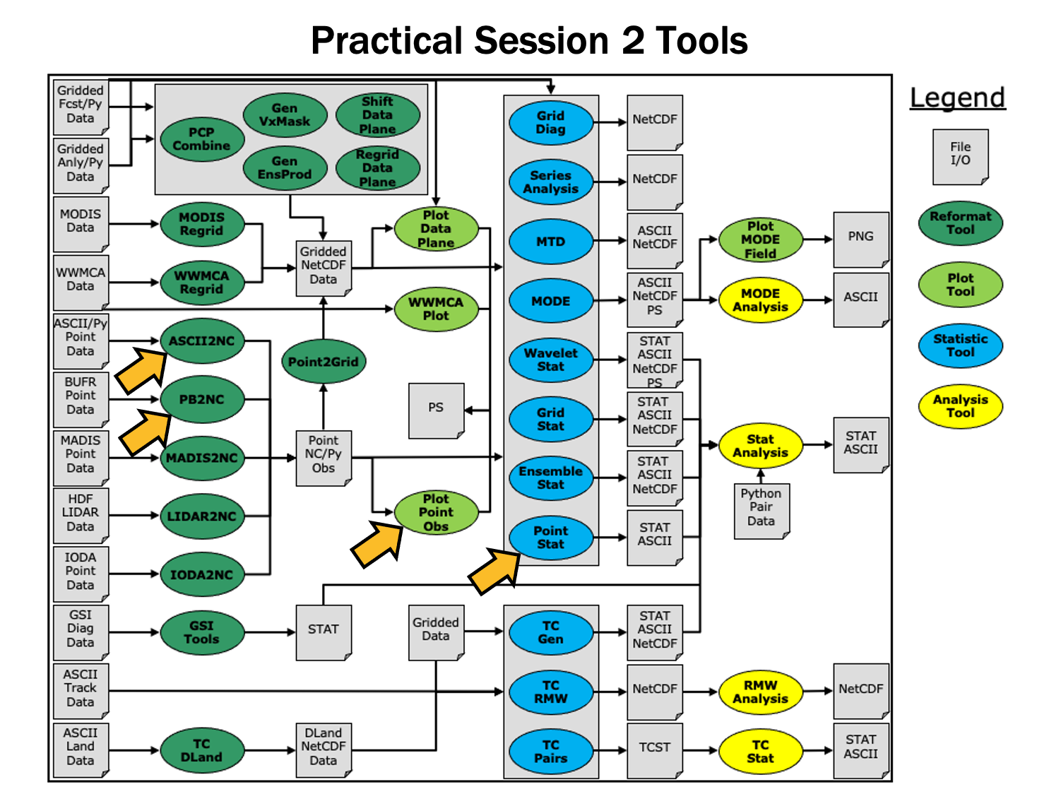 You may navigate through this tutorial by following the links at the bottom of each page or by using the menu navigation.
Since you already set up your runtime environment in Session 1, you should be ready to go! To be sure, run through the following instructions to check that your environment is set correctly.
Prerequisites: Verify Environment is Set Correctly
Before running the tutorial instructions, you will need to ensure that you have a few environment variables set up correctly. If they are not set correctly, the tutorial instructions will not work properly.
EDIT AFTER COPYING and BEFORE HITTING RETURN!
source METplus-5.0.0_TutorialSetup.sh
echo ${METPLUS_BUILD_BASE}
echo ${MET_BUILD_BASE}
echo ${METPLUS_DATA}
ls ${METPLUS_TUTORIAL_DIR}
ls ${METPLUS_BUILD_BASE}
ls ${MET_BUILD_BASE}
ls ${METPLUS_DATA}
METPLUS_BUILD_BASE is the full path to the METplus installation (/path/to/METplus-X.Y)
MET_BUILD_BASE is the full path to the MET installation (/path/to/met-X.Y)
METPLUS_DATA is the location of the sample test data directory
ls ${METPLUS_BUILD_BASE}/ush/run_metplus.py
See the instructions in Session 1 for more information.
You are now ready to move on to the next section.
MET Tool: PB2NC
MET Tool: PB2NC
PB2NC Tool: General
PB2NC Functionality
The PB2NC tool is used to stratify (i.e. subset) the contents of an input PrepBufr point observation file and reformat it into NetCDF format for use by the Point-Stat or Ensemble-Stat tool. In this session, we will run PB2NC on a PrepBufr point observation file prior to running Point-Stat. Observations may be stratified by variable type, PrepBufr message type, station identifier, a masking region, elevation, report type, vertical level category, quality mark threshold, and level of PrepBufr processing. Stratification is controlled by a configuration file and discussed on the next page.
The PB2NC tool may be run on both PrepBufr and Bufr observation files. As of met-6.1, support for Bufr is limited to files containing embedded tables. Support for Bufr files using external tables will be added in a future release.
For more information about the PrepBufr format, visit:
https://emc.ncep.noaa.gov/emc/pages/infrastructure/bufrlib.php
For information on where to download PrepBufr files, visit:
https://dtcenter.org/community-code/model-evaluation-tools-met/input-data
PB2NC Usage
| Usage: pb2nc | ||
| prepbufr_file | input prepbufr path/filename | |
| netcdf_file | output netcdf path/filename | |
| config_file | configuration path/filename | |
| [-pbfile prepbufr_file] | additional input files | |
| [-valid_beg time] | Beginning of valid time window [YYYYMMDD_[HH[MMSS]]] | |
| [-valid_end time] | End of valid time window [YYYYMMDD_[HH[MMSS]]] | |
| [-nmsg n] | Number of PrepBufr messages to process | |
| [-index] | List available observation variables by message type (no output file) | |
| [-dump path] | Dump entire contents of PrepBufr file to directory | |
| [-obs_var var] | Sets the variable list to be saved from input BUFR files | |
| [-log file] | Outputs log messages to the specified file | |
| [-v level] | Level of logging | |
| [-compression level] | NetCDF file compression |
At a minimum, the input prepbufr_file, the output netcdf_file, and the configuration config_file must be passed in on the command line. Also, you may use the -pbfile command line argument to run PB2NC using multiple input PrepBufr files, likely adjacent in time.
When running PB2NC on a new dataset, users are advised to run with the -index option to list the observation variables that are present in that file.
Configure
Configure
PB2NC Tool: Configure
cd ${METPLUS_TUTORIAL_DIR}/output/met_output/pb2nc
The behavior of PB2NC is controlled by the contents of the configuration file passed to it on the command line. The default PB2NC configuration may be found in the data/config/PB2NCConfig_default file.
The configurable items for PB2NC are used to filter out the PrepBufr observations that should be retained or derived. You may find a complete description of the configurable items in the pb2nc configuration file section of the MET User's Guide or in the Configuration File Overview.
For this tutorial, edit the PB2NCConfig_tutorial_run1 file as follows:
- Set:
message_type = [ "ADPUPA", "ADPSFC" ];to retain only those 2 message types. Message types are described in:
http://www.emc.ncep.noaa.gov/mmb/data_processing/prepbufr.doc/table_1.htm - Set:
obs_window = {
beg = -1800;
end = 1800;
}so that only observations within 1800 second (30 minutes) of the file time will be retained.
- Set:
mask = {
grid = "G212";
poly = "";
}to retain only those observations residing within NCEP Grid 212, on which the forecast data resides.
- Set:
obs_bufr_var = [ "QOB", "TOB", "UOB", "VOB", "D_WIND", "D_RH" ];to retain observations for specific humidity, temperature, the u-component of wind, and the v-component of wind and to derive observation values for wind speed and relative humidity.
While we are request these observation variable names from the input file, the following corresponding strings will be written to the output file: SPFH, TMP, UGRD, VGRD, WIND, RH. This mapping of input PrepBufr variable names to output variable names is specified by the obs_prepbufr_map config file entry. This enables the new features in the current version of MET to be backward compatible with earlier versions.
Run
Run
PB2NC Tool: Run
${METPLUS_DATA}/met_test/data/sample_obs/prepbufr/ndas.t00z.prepbufr.tm12.20070401.nr \
tutorial_pb_run1.nc \
PB2NCConfig_tutorial_run1 \
-v 2
PB2NC is now filtering the observations from the PrepBufr file using the configuration settings we specified and writing the output to the NetCDF file name we chose. This should take a few minutes to run. As it runs, you should see several status messages printed to the screen to indicate progress. You may use the -v command line option to turn off (-v 0) or change the amount of log information printed to the screen.
If you'd like to filter down the observations further, you may want to narrow the time window or modify other filtering criteria. We will do that after inspecting the resultant NetCDF file.
Output
Output
PB2NC Tool: Output
When PB2NC is finished, you may view the output NetCDF file it wrote using the ncdump utility.
In the NetCDF header, you'll see that the file contains nine dimensions and nine variables. The obs_arr variable contains the actual observation values. The obs_qty variable contains the corresponding quality flags. The four header variables (hdr_typ, hdr_sid, hdr_vld, hdr_arr) contain information about the observing locations.
The obs_var, obs_unit, and obs_desc variables describe the observation variables contained in the output. The second entry of the obs_arr variable (i.e. var_id) lists the index into these array for each observation. For example, for observations of temperature, you'd see TMP in obs_var, KELVIN in obs_unit, and TEMPERATURE OBSERVATION in obs_desc. For observations of temperature in obs_arr, the second entry (var_id) would list the index of that temperature information.
Plot-Point-Obs
The plot_point_obs tool plots the location of these NetCDF point observations. Just like plot_data_plane is useful to visualize gridded data, run plot_point_obs to make sure you have point observations where you expect.
tutorial_pb_run1.nc \
tutorial_pb_run1.ps
Each red dot in the plot represents the location of at least one observation value. The plot_point_obs tool has additional command line options for filtering which observations get plotted and the area to be plotted.
By default, the points are plotted on the full globe.
tutorial_pb_run1.nc \
tutorial_pb_run1_zoom.ps \
-data_file ${METPLUS_DATA}/met_test/data/sample_fcst/2007033000/nam.t00z.awip1236.tm00.20070330.grb
MET extracts the grid information from the first record of that GRIB file and plots the points on that domain.
The plot_data_plane tool can be run on the NetCDF output of any of the MET point observation pre-processing tools (pb2nc, ascii2nc, madis2nc, and lidar2nc).
Reconfigure and Rerun
Reconfigure and Rerun
PB2NC Tool: Reconfigure and Rerun
Now we'll rerun PB2NC, but this time we'll tighten the observation acceptance criteria.
- Set:
message_type = [];to retain all message types.
- Set:
obs_window = {
beg = -25*30;
end = 25*30;
}so that only observations 25 minutes before and 25 minutes after the top of the hour are retained.
- Set:
quality_mark_thresh = 1;to retain only the observations marked "Good" by the NCEP quality control system.
${METPLUS_DATA}/met_test/data/sample_obs/prepbufr/ndas.t00z.prepbufr.tm12.20070401.nr \
tutorial_pb_run2.nc \
PB2NCConfig_tutorial_run2 \
-v 2
The majority of the observations were rejected because their valid time no longer fell inside the tighter obs_window setting.
When configuring PB2NC for your own projects, you should err on the side of keeping more data rather than less. As you'll see, the grid-to-point verification tools (Point-Stat and Ensemble-Stat) allow you to further refine which point observations are actually used in the verification. However, keeping a lot of point observations that you'll never actually use will make the data files larger and slightly slow down the verification. For example, if you're using a Global Data Assimilation (GDAS) PREPBUFR file to verify a model over Europe, it would make sense to only keep those point observations that fall within your model domain.
METplus Use Case: PB2NC
METplus Use Case: PB2NC
METplus Use Case: PB2NC
This use case utilizes the MET PB2NC tool.
Optional: Refer to the MET Users Guide for a description of the MET tools used in this use case.
Optional: Refer to the METplus Config Glossary section of the METplus Users Guide for a reference to METplus variables used in this use case.
-
Review the settings in the PB2NC.conf file:
Note that the input directory PB2NC_INPUT_DIR is set to a path relative to {INPUT_BASE} and the output directory PB2NC_OUTPUT_DIR is set to a path relative to {OUTPUT_BASE}:
...
PB2NC_INPUT_DIR = {INPUT_BASE}/met_test/data/sample_obs/prepbufr
...
PB2NC_OUTPUT_DIR = {OUTPUT_BASE}/pb2nc
{PARM_BASE} is set automatically by METplus. The wrapped MET config file for PB2NC is set relative to {PARM_BASE} in PB2NC_CONFIG_FILE:
Values for the MET tool PB2NC are passed in from METplus config files, including PB2NC.conf
//
// PB2NC configuration file.
//
// For additional information, see the MET_BASE/config/README file.
// ////////////////////////////////////////////////////////////////////////////////
//
// PrepBufr message type
//
${PB2NC_MESSAGE_TYPE} ;
//
// Mapping of message type group name to comma-separated list of values
// Derive PRMSL only for SURFACE message types
//
message_type_group_map = [
{ key = "SURFACE"; val = "ADPSFC,SFCSHP,MSONET"; },
{ key = "ANYAIR"; val = "AIRCAR,AIRCFT"; },
{ key = "ANYSFC"; val = "ADPSFC,SFCSHP,ADPUPA,PROFLR,MSONET"; },
{ key = "ONLYSF"; val = "ADPSFC,SFCSHP" }
];
No modifications are needed to run the PB2NC METplus tool.
-
Run the PB2NC use case:
${METPLUS_BUILD_BASE}/parm/use_cases/met_tool_wrapper/PB2NC/PB2NC.conf \
${METPLUS_TUTORIAL_DIR}/tutorial.conf \
config.OUTPUT_BASE=${METPLUS_TUTORIAL_DIR}/output/PB2NC
-
Review the output file:
The following is the statistical output and file generated from the command:
- sample_pb.nc
MET Tool: ASCII2NC
MET Tool: ASCII2NC
ASCII2NC Tool: General
ASCII2NC Functionality
The ASCII2NC tool reformats ASCII point observations into the intermediate NetCDF format that Point-Stat and Ensemble-Stat read. ASCII2NC simply reformats the data and does much less filtering of the observations than PB2NC does. ASCII2NC supports a simple 11-column format, described below, the Little-R format often used in data assimilation, SURFace RADiation (SURFRAD) data, Western Wind and Solar Integration Studay (WWSIS) data, and AErosol RObotic NEtwork (Aeronet) data versions 2 and 3 format. MET version 9.0 added support for passing observations to ASCII2NC using a Python script. Future version of MET may be enhanced to support additional commonly used ASCII point observation formats based on community input.
MET Point Observation Format
The MET point observation format consists of one observation value per line. Each input observation line should consist of the following 11 columns of data:
- Message_Type
- Station_ID
- Valid_Time in YYYYMMDD_HHMMSS format
- Lat in degrees North
- Lon in degrees East
- Elevation in meters above sea level
- Variable_Name for this observation (or GRIB_Code for backward compatibility)
- Level as the pressure level in hPa or accumulation interval in hours
- Height in meters above sea level or above ground level
- QC_String quality control string
- Observation_Value
It is the user's responsibility to get their ASCII point observations into this format.
ASCII2NC Usage
| Usage: ascii2nc | ||
| ascii_file1 [...] | One or more input ASCII path/filename | |
| netcdf_file | Output NetCDF path/filename | |
| [-format ASCII_format] | Set to met_point, little_r, surfrad, wwsis, aeronet, aeronetv2, aeronetv3, or python | |
| [-config file] | Configuration file to specify how observation data should be summarized | |
| [-mask_grid string] | Named grid or a gridded data file for filtering point observations spatially | |
| [-mask_poly file] | Polyline masking file for filtering point observations spatially | |
| [-mask_sid file|list] | Specific station ID's to be used in an ASCII file or comma-separted list | |
| [-log file] | Outputs log messages to the specified file | |
| [-v level] | Level of logging | |
| [-compress level] | NetCDF compression level |
At a minimum, the input ascii_file and the output netcdf_file must be passed on the command line. ASCII2NC interrogates the data to determine it's format, but the user may explicitly set it using the -format command line option. The -mask_grid, -mask_poly, and -mask_sid options can be used to filter observations spatially.
Run
Run
ASCII2NC Tool: Run
cd ${METPLUS_TUTORIAL_DIR}/output/met_output/ascii2nc
Since ASCII2NC performs a simple reformatting step, typically no configuration file is needed. However, when processing high-frequency (1 or 3-minute) SURFRAD data, a configuration file may be used to define a time window and summary metric for each station. For example, you might compute the average observation value +/- 15 minutes at the top of each hour for each station. In this example, we will not use a configuration file.
The sample ASCII observations in the MET tarball are still identified by GRIB code rather than the newer variable name option.
For example, 52 corresponds to RH:
${METPLUS_DATA}/met_test/data/sample_obs/ascii/sample_ascii_obs.txt \
tutorial_ascii.nc \
-v 2
ASCII2NC should perform this reformatting step very quickly since the sample file only contains data for 5 stations.
Output
Output
ASCII2NC Tool: Output
When ASCII2NC is finished, you may view the output NetCDF file it wrote using the ncdump utility.
The NetCDF header should look nearly identical to the output of the NetCDF output of PB2NC. You can see the list of stations for which we have data by inspecting the hdr_sid_table variable:
This ASCII data only contains observations at a few locations.
tutorial_ascii.nc \
tutorial_ascii.ps \
-data_file ${METPLUS_DATA}/met_test/data/sample_fcst/2007033000/nam.t00z.awip1236.tm00.20070330.grb \
-v 3
Next, we'll use the NetCDF output of PB2NC and ASCII2NC to perform Grid-to-Point verification using the Point-Stat tool.
METplus Use Case: ASCII2NC with Python Embedding
METplus Use Case: ASCII2NC with Python Embedding
METplus Use Case: ASCII2NC with Python Embedding
This use case utilizes the MET ASCII2NC tool to demonstrate Python Embedding. Python embedding is a novel capability within METplus that allows a user to place a Python script into a METplus workflow. For example, if a user has a data format that is unsupported by the MET tools then a user could write their own Python file reader, and hand off the data to the MET tools within a workflow.
The data utilized in this use case are hypothetical accumulated precipitation data in ASCII format.
Optional: Refer to the MET Users Guide for a description of the MET tools used in this use case.
Optional: Refer to the MET Users Guide Appendix F: Python Embedding for details on how Python embedding works for MET tools.
Optional: Refer to the METplus Config Glossary section of the METplus Users Guide for a reference to METplus variables used in this use case.
-
View the template Python Embedding scripts available with MET
MET includes example scripts for reading point data and gridded data (all in ASCII format). These can be used by users as a jumping-off point for developing their own Python embedding scripts, and are also used by this use case and other METplus use cases that demonstrate Python Embedding
met_point_obs.py
read_ascii_mpr.py
read_ascii_numpy_grid.py
read_ascii_numpy.py
read_ascii_point.py
read_ascii_xarray.py
read_met_point_obs.py
In this use case, read_ascii_point.py is used to read the sample accumulated precipitation data and serve them to ASCII2NC to format into the MET 11-column netCDF format.
-
Inspect a sample of the accumulated precipitation point data being read with Python.
These data are already in the 11-column format that MET requires, so using Python Embedding is fairly straightforward. If your data do not follow this format, some pre-processing of the data will be required to align your data to the required format. To learn more about what the 11 columns are and what MET expects each column to represent, please reference this table from the MET users guide.
-
Inspect the Python Embedding script being used in this use case
Since the sample data are point data, the Python module Pandas is utilized to read the ASCII data, assign column names that match the MET 11-column format, and then pass the data to the MET ASCII2NC tool.
-
Run the ASCII2NC Python Embedding use case:
${METPLUS_BUILD_BASE}/parm/use_cases/met_tool_wrapper/ASCII2NC/ASCII2NC_python_embedding.conf \
${METPLUS_TUTORIAL_DIR}/tutorial.conf \
config.OUTPUT_BASE=${METPLUS_TUTORIAL_DIR}/output/ASCII2NC_python_embedding
This command utilizes the METplus wrappers to execute a Python script to read in the ASCII data and pass them off to ASCII2NC to write to a netCDF file. While the Python script called here is simply for demonstration purposes, your Python script could serve to perform various data manipulation and formatting, or reading of proprietary or unsupported file formats to end up with a netCDF file compatible with the MET tools.
-
Review the Output Files
You should see the output netCDF file (ascii2nc_python.nc), which conforms to the 11-column format required by the MET tools.
-
Let's Write Some Python!
Copy the METplus use configuration file to your current working directory:
Copy the Python Embedding script to your current working directory and rename it to my_ascii_point.py:
Open the Python Embedding script in a text editor of your choice, and add the following on line 7 of the file (make sure the indentation matches the previous line):
Add on line 7:
Save the Python Embedding script.
-
Modify the METplus Use Case Configuration File to Use Your Python Script
Open the METplus use case file in a text editor of your choice and modify line 43 to use your Python script:
Change line 43 to:
The Python script contains an import of met_point_obs. This is found automatically by the read_ascii_point.py script because it is in the same share/met/python directory. Since you are calling my_ascii_point.py from your tutorial directory, you will have to set the PYTHONPATH to include the share/met/python directory so the import succeeds.
Add the following to the very end of ${METPLUS_TUTORIAL_DIR}/ASCII2NC_python_embedding.conf:
PYTHONPATH={MET_INSTALL_DIR}/share/met/python:$PYTHONPATH
Save the METplus use case configuration file.
-
Re-run the Use Case, and See If Your Python Code Is Used
${METPLUS_TUTORIAL_DIR}/ASCII2NC_python_embedding.conf \
${METPLUS_TUTORIAL_DIR}/tutorial.conf \
config.OUTPUT_BASE=${METPLUS_TUTORIAL_DIR}/output/ASCII2NC_python_embedding
-
Look for Your Python Print Statement In the METplus Log File
The 2nd last log message printed to the screen will contain the full path to the log file that was created for this run. Copy this path and run less to view the log file. It will look something like this:
(NOTE: Replace YYYYMMDDHHMMSS with the time and date appended to the log file from the run in step 8). You should see the print statement written to the log file, showing that your modifications were used by METplus and ASCII2NC!
MET Tool: Point-Stat
MET Tool: Point-Stat
Point-Stat Tool: General
Point-Stat Functionality
The Point-Stat tool provides verification statistics for comparing gridded forecasts to observation points, as opposed to gridded analyses like Grid-Stat. The Point-Stat tool matches gridded forecasts to point observation locations using one or more configurable interpolation methods. The tool then computes a configurable set of verification statistics for these matched pairs. Continuous statistics are computed over the raw matched pair values. Categorical statistics are generally calculated by applying a threshold to the forecast and observation values. Confidence intervals, which represent a measure of uncertainty, are computed for all of the verification statistics.
Point-Stat Usage
| Usage: point_stat | ||
| fcst_file | Input gridded file path/name | |
| obs_file | Input NetCDF observation file path/name | |
| config_file | Configuration file | |
| [-point_obs file] | Additional NetCDF observation files to be used (optional) | |
| [-obs_valid_beg time] | Sets the beginning of the matching time window in YYYYMMDD[_HH[MMSS]] format (optional) | |
| [-obs_valid_end time] | Sets the end of the matching time window in YYYYMMDD[_HH[MMSS]] format (optional) | |
| [-outdir path] | Overrides the default output directory (optional) | |
| [-log file] | Outputs log messages to the specified file (optional) | |
| [-v level] | Level of logging (optional) |
At a minimum, the input gridded fcst_file, the input NetCDF obs_file (output of PB2NC, ASCII2NC, MADIS2NC, and LIDAR2NC, last two not covered in these exercises), and the configuration config_file must be passed in on the command line. You may use the -point_obs command line argument to specify additional NetCDF observation files to be used.
Configure
Configure
Point-Stat Tool: Configure
cd ${METPLUS_TUTORIAL_DIR}/output/met_output/point_stat
The behavior of Point-Stat is controlled by the contents of the configuration file passed to it on the command line. The default Point-Stat configuration file may be found in the data/config/PointStatConfig_default file.
The configurable items for Point-Stat are used to specify how the verification is to be performed. The configurable items include specifications for the following:
- The forecast fields to be verified at the specified vertical levels.
- The type of point observations to be matched to the forecasts.
- The threshold values to be applied.
- The areas over which to aggregate statistics - as predefined grids, lat/lon polylines, or individual stations.
- The confidence interval methods to be used.
- The interpolation methods to be used.
- The types of verification methods to be used.
- Set:
fcst = {
message_type = [ "ADPUPA" ];
field = [
{
name = "TMP";
level = [ "P850-1050", "P500-850" ];
cat_thresh = [ <=273, >273 ];
}
];
}
obs = fcst;to verify temperature over two different pressure ranges against ADPUPA observations using the thresholds specified.
- Set:
ci_alpha = [ 0.05, 0.10 ];to compute confidence intervals using both a 5% and a 10% level of certainty.
- Set:
output_flag = {
fho = BOTH;
ctc = BOTH;
cts = STAT;
mctc = NONE;
mcts = NONE;
cnt = BOTH;
sl1l2 = STAT;
sal1l2 = NONE;
vl1l2 = NONE;
val1l2 = NONE;
pct = NONE;
pstd = NONE;
pjc = NONE;
prc = NONE;
ecnt = NONE;
eclv = BOTH;
mpr = BOTH;
}to indicate that the forecast-hit-observation (FHO) counts, contingency table counts (CTC), contingency table statistics (CTS), continuous statistics (CNT), partial sums (SL1L2), economic cost/loss value (ECLV), and the matched pair data (MPR) line types should be output. Setting SL1L2 and CTS to STAT causes those lines to only be written to the output .stat file, while setting others to BOTH causes them to be written to both the .stat file and the optional LINE_TYPE.txt file.
- Set:
output_prefix = "run1";to customize the output file names for this run.
Note that in the mask dictionary, the grid entry is set to FULL. This instructs Point-Stat to compute statistics over the entire input model domain. Setting grid to FULL has this special meaning.
Run
Run
Point-Stat Tool: Run
Next, run Point-Stat to compare a GRIB forecast to the NetCDF point observation output of the ASCII2NC tool.
${METPLUS_DATA}/met_test/data/sample_fcst/2007033000/nam.t00z.awip1236.tm00.20070330.grb \
../ascii2nc/tutorial_ascii.nc \
PointStatConfig_tutorial_run1 \
-outdir . \
-v 2
Point-Stat is now performing the verification tasks we requested in the configuration file. It should take less than a minute to run. You should see several status messages printed to the screen to indicate progress.
If you receive a syntax error such as the one listed below, review PointStatConfig_tutorial_run1 for an extra comma after the "}" on line number 59
cat_thresh = [ >273.0 ];
}, <---Remove the comma
DEBUG 1: Default Config File: /usr/local/met-9.0/share/met/config/PointStatConfig_default
DEBUG 1: User Config File: PointStatConfig_tutorial_run1
ERROR :
ERROR : yyerror() -> syntax error in file "/tmp/met_config_26760_0"
ERROR :
ERROR : line = 59
ERROR :
ERROR : column = 0
ERROR :
ERROR : text = "]"
ERROR :
ERROR :
ERROR : ];
ERROR : _____
ERROR :
Notice the more detailed information about which observations were used for each verification task. If you run Point-Stat and get fewer matched pairs than you expected, try using the -v 3 option to see why the observations were rejected.
Output
Output
Point-Stat Tool: Output
The output of Point-Stat is one or more ASCII files containing statistics summarizing the verification performed. Since we wrote output to the current directory, it should now contain 6 ASCII files that begin with the point_stat_ prefix, one each for the FHO, CTC, CNT, ECLV, and MPR types, and a sixth for the STAT file. The STAT file contains all of the output statistics while the other ASCII files contain the exact same data organized by line type.
- In the kwrite editor, select Settings->Configure Editor, de-select Dynamic Word Wrap and click OK.
- In the vi editor, type the command :set nowrap. To set this as the default behavior, run the following command:
echo "set nowrap" >> ~/.exrc
- This is a simple ASCII file consisting of several rows of data.
- Each row contains data for a single verification task.
- The FCST_LEAD, FCST_VALID_BEG, and FCST_VALID_END columns indicate the timing information of the forecast field.
- The OBS_LEAD, OBS_VALID_BEG, and OBS_VALID_END columns indicate the timing information of the observation field.
- The FCST_VAR, FCST_UNITS, FCST_LEV, OBS_VAR, OBS_UNITS, and OBS_LEV columns indicate the two parts of the forecast and observation fields set in the configure file.
- The OBTYPE column indicates the PrepBufr message type used for this verification task.
- The VX_MASK column indicates the masking region over which the statistics were accumulated.
- The INTERP_MTHD and INTERP_PNTS columns indicate the method used to interpolate the forecast data to the observation location.
- The FCST_THRESH and OBS_THRESH columns indicate the thresholds applied to FCST_VAR and OBS_VAR.
- The COV_THRESH column is not applicable here and will always have NA when using point_stat.
- The ALPHA column indicates the alpha used for confidence intervals.
- The LINE_TYPE column indicates that these are CTC contingency table count lines.
- The TOTAL column indicates the total number of matched pairs.
- The remaining columns contain the counts for the contingency table computed by applying the threshold to the forecast/observation matched pairs. The FY_OY (forecast: yes, observation: yes), FY_ON (forecast: yes, observation: no), FN_OY (forecast: no, observation: yes), and FN_ON (forecast: no, observation: no) columns indicate those counts.
- What do you notice about the structure of the contingency table counts with respect to the two thresholds used? Does this make sense?
- Does the model appear to resolve relatively cold surface temperatures?
- Based on these observations, are temperatures >273 relatively rare or common in the P850-500 range? How can this affect the ability to get a good score using contingency table statistics? What about temperatures <=273 at the surface?
- The columns prior to LINE_TYPE contain the same data as the previous file we viewed.
- The LINE_TYPE column indicates that these are CNT continuous lines.
- The remaining columns contain continuous statistics derived from the raw forecast/observation pairs. See the CNT OUTPUT FORMAT section in the Point-Stat section of the MET User's Guide for a thorough description of the output.
- Again, confidence intervals are given for each of these statistics as described above.
- What conclusions can you draw about the model's performance at each level using continuous statistics? Justify your answer. Did you use a single metric in your evaluation? Why or why not?
- Comparing the first line with an alpha value of 0.05 to the second line with an alpha value of 0.10, how does the level of confidence change the upper and lower bounds of the confidence intervals (CIs)?
- Similarly, comparing the first line with few numbers of matched pairs in the TOTAL column to the third line with more, how does the sample size affect how you interpret your results?
- The columns prior to LINE_TYPE contain the same data as the previous file we viewed.
- The LINE_TYPE column indicates that these are FHO forecast-hit-observation rate lines.
- The remaining columns are similar to the contingency table output and contain the total number of matched pairs, the forecast rate, the hit rate, and observation rate.
- The forecast, hit, and observation rates should back up your answer to the third question about the contingency table output.
- The columns prior to LINE_TYPE contain the same data as the previous file we viewed.
- The LINE_TYPE column indicates that these are MPR matched pair lines.
- The remaining columns are similar to the contingency table output and contain the total number of matched pairs, the matched pair index, the latitude, longitude, and elevation of the observation, the forecasted value, the observed value, and the climatological value (if applicable).
- There is a lot of data here and it is recommended that the MPR line_type is used only to verify the tool is working properly.
Reconfigure
Reconfigure
Point-Stat Tool: Reconfigure
Now we'll reconfigure and rerun Point-Stat.
This time, we'll use two dictionary entries to specify the forecast field in order to set different thresholds for each vertical level. Point-Stat may be configured to verify as many or as few model variables and vertical levels as you desire.
- Set:
fcst = {
field = [
{
name = "TMP";
level = [ "Z2" ];
cat_thresh = [ >273, >278, >283, >288 ];
},
{
name = "TMP";
level = [ "P750-850" ];
cat_thresh = [ >278 ];
}
];
}
obs = fcst;to verify 2-meter temperature and temperature fields between 750hPa and 850hPa, using the thresholds specified.
- Set:
message_type = ["ADPUPA","ADPSFC"];
sid_inc = [];
sid_exc = [];
obs_quality = [];
duplicate_flag = NONE;
obs_summary = NONE;
obs_perc_value = 50;to include the Upper Air (UPA) and Surface (SFC) observations in the evaluation
- Set:
mask = {
grid = [ "G212" ];
poly = [ "MET_BASE/poly/EAST.poly",
"MET_BASE/poly/WEST.poly" ];
sid = [];
llpnt = [];
}to compute statistics over the NCEP Grid 212 region and over the Eastern and Western United States, as defined by the polylines specified.
- Set:
interp = {
vld_thresh = 1.0;
shape = SQUARE;
type = [
{
method = NEAREST;
width = 1;
},
{
method = DW_MEAN;
width = 5;
}
];
}to indicate that the forecast values should be interpolated to the observation locations using the nearest neighbor method and by computing a distance-weighted average of the forecast values over the 5 by 5 box surrounding the observation location.
- Set:
output_flag = {
fho = BOTH;
ctc = BOTH;
cts = BOTH;
mctc = NONE;
mcts = NONE;
cnt = BOTH;
sl1l2 = BOTH;
sal1l2 = NONE;
vl1l2 = NONE;
val1l2 = NONE;
pct = NONE;
pstd = NONE;
pjc = NONE;
prc = NONE;
ecnt = NONE;
eclv = BOTH;
mpr = BOTH;
}to switch the SL1L2 and CTS output to BOTH and generate the optional ASCII output files for them.
- Set:
output_prefix = "run2";to customize the output file names for this run.
- 2 fields: TMP/Z2 and TMP/P750-850
- 2 observing message types: ADPUPA and ADPSFC
- 3 masking regions: G212, EAST.poly, and WEST.poly
- 2 interpolations: UW_MEAN width 1 (nearest-neighbor) and DW_MEAN width 5
Multiplying 2 * 2 * 3 * 2 = 24. So in this example, Point-Stat will accumulate matched forecast/observation pairs into 24 groups. However, some of these groups will result in 0 matched pairs being found. To each non-zero group, the specified threshold(s) will be applied to compute contingency tables.
Rerun
Rerun
Point-Stat Tool: Rerun
Next, run Point-Stat to compare a GRIB forecast to the NetCDF point observation output of the PB2NC tool, as opposed to the much smaller ASCII2NC output we used in the first run.
${METPLUS_DATA}/met_test/data/sample_fcst/2007033000/nam.t00z.awip1236.tm00.20070330.grb \
../pb2nc/tutorial_pb_run1.nc \
PointStatConfig_tutorial_run2 \
-outdir . \
-v 2
Point-Stat is now performing the verification tasks we requested in the configuration file. It should take a minute or two to run. You should see several status messages printed to the screen to indicate progress. Note the number of matched pairs found for each verification task, some of which are 0.
Plot-Data-Plane Tool
In this step, we have verified 2-meter temperature. The Plot-Data-Plane tool within MET provides a way to visualize the gridded data fields that MET can read.
${METPLUS_DATA}/met_test/data/sample_fcst/2007033000/nam.t00z.awip1236.tm00.20070330.grb \
nam.t00z.awip1236.tm00.20070330_TMPZ2.ps \
'name="TMP"; level="Z2";'
Plot-Data-Plane requires an input gridded data file, an output postscript image file name, and a configuration string defining which 2-D field is to be plotted.
-
Set the title to 2-m Temperature.
-
Set the plotting range as 250 to 305.
-
Use the color table named ${MET_BUILD_BASE}/share/met/colortables/NCL_colortables/wgne15.ctable
Next, we'll take a look at the Point-Stat output we just generated.
See the usage statement for all MET tools using the --help command line option or with no options at all.
Output
Output
Point-Stat Tool: Output
The format for the CTC, CTS, and CNT line types are the same. However, the numbers will be different as we used a different set of observations for the verification.
- The columns prior to LINE_TYPE contain header information.
- The LINE_TYPE column indicates that these are CTS lines.
- The remaining columns contain statistics derived from the threshold contingency table counts. See the point_stat output section of the MET User's Guide for a thorough description of the output.
- Confidence intervals are given for each of these statistics, computed using either one or two methods. The columns ending in _NCL(normal confidence lower) and _NCU (normal confidence upper) give lower and upper confidence limits computed using assumptions of normality. The columns ending in _BCL (bootstrap confidence lower) and _BCU (bootstrap confidence upper) give lower and upper confidence limits computed using bootstrapping.
- The columns prior to LINE_TYPE contain header information.
- The LINE_TYPE column indicates these are SL1L2 partial sums lines.
Lastly, the point_stat_run2_360000L_20070331_120000V.stat file contains all of the same data we just viewed but in a single file. The Stat-Analysis tool, which we'll use later in this tutorial, searches for the .stat output files by default but can also read the .txt output files.
METplus Use Case: PointStat
METplus Use Case: PointStat
METplus Use Case: PointStat
This use case utilizes the MET Point-Stat tool.
Optional: Refer to the MET Users Guide for a description of the MET tools used in this use case.
Optional: Refer to the METplus Config Glossary section of the METplus Users Guide for a reference to METplus variables used in this use case.
-
View Configuration File
The forecast and observations directories are specified in relation to INPUT_BASE (${METPLUS_DATA}), while the output directory is given in relation to {OUTPUT_BASE} (${METPLUS_TUTORIAL_DIR}/output).
OBS_POINT_STAT_INPUT_DIR = {INPUT_BASE}/met_test/out/pb2nc
...
POINT_STAT_OUTPUT_DIR = {OUTPUT_BASE}/point_stat
Using the PointStat configuration file, you should be able to run the use case using the sample input data set without any other changes.
-
Run the PointStat use case:
${METPLUS_BUILD_BASE}/parm/use_cases/met_tool_wrapper/PointStat/PointStat.conf \
${METPLUS_TUTORIAL_DIR}/tutorial.conf \
config.OUTPUT_BASE=${METPLUS_TUTORIAL_DIR}/output/PointStat
-
Review the output file:
The following is the statistical output and file are generated from the command:
- point_stat_360000L_20070331_120000V.stat
-
Update configuration file and re-run
vi ${METPLUS_TUTORIAL_DIR}/user_config/PointStat_tutorial.conf
BOTH_VAR1_NAME = TMP
BOTH_VAR1_LEVELS = P750-900
BOTH_VAR1_THRESH = <=273, >273
BOTH_VAR2_NAME = UGRD
BOTH_VAR2_LEVELS = Z10
BOTH_VAR2_THRESH = >=5
BOTH_VAR3_NAME = VGRD
BOTH_VAR3_LEVELS = Z10
BOTH_VAR3_THRESH = >=5
-
Rerun the use-case and compare the output
${METPLUS_TUTORIAL_DIR}/user_config/PointStat_tutorial.conf \
${METPLUS_TUTORIAL_DIR}/tutorial.conf \
config.OUTPUT_BASE=${METPLUS_TUTORIAL_DIR}/output/PointStat
${METPLUS_TUTORIAL_DIR}/output/PointStat/point_stat/point_stat_360000L_20070331_120000V.stat \
${METPLUS_TUTORIAL_DIR}/output/PointStat/point_stat/point_stat_run2_360000L_20070331_120000V.stat
METplus Use Case: PointStat - Standard Verification of Global Upper Air
METplus Use Case: PointStat - Standard Verification of Global Upper Air
METplus Use Case: PointStat - Standard Verification of Global Upper Air
This use case utilizes the MET Point-Stat tool.
Optional: Refer to the MET Users Guide for a description of the MET tools used in this use case.
Optional: Refer to the METplus Config Glossary section of the METplus Users Guide for a reference to METplus variables used in this use case.
-
View Configuration File
[statistics tool(s)]_fcst[Model]_obs[Point Data or Analysis]_[other decriptors including file format].conf
This use-case includes running two tools, PB2NC to extract the observations and then Point-Stat to compute statistics. Note the specification of wrappers to run is given in the PROCESS_LIST at the top of the file.
PROCESS_LIST = PB2NC, PointStat
BOTH_VAR1_LEVELS = P1000, P925, P850, P700, P500, P400, P300, P250, P200, P150, P100, P50, P20, P10
BOTH_VAR2_NAME = RH
BOTH_VAR2_LEVELS = P1000, P925, P850, P700, P500, P400, P300
...
BOTH_VAR5_NAME = HGT
BOTH_VAR5_LEVELS = P1000, P950, P925, P850, P700, P500, P400, P300, P250, P200, P150, P100, P50, P20, P10
Using the PointStat configuration file, you should be able to run the use case using the sample input data set without any other changes.
-
Run the PointStat use case:
${METPLUS_BUILD_BASE}/parm/use_cases/model_applications/medium_range/PointStat_fcstGFS_obsGDAS_UpperAir_MultiField_PrepBufr.conf \
${METPLUS_TUTORIAL_DIR}/tutorial.conf \
config.OUTPUT_BASE=${METPLUS_TUTORIAL_DIR}/output/PointStat_UpperAir
This may take a few minutes to run.
-
Review the output files:
If you scroll down to the middle of the file, you will notice the statistics line-type starts alternating from SL1L2 (partial_sums for continuous statistics) to VL1L2 (partial_sums for vector continuous statistics). If you scroll over, you will see that the lines are different lengths. The MET Users' Guide explains what statistics are reported in each line. See point-stat output in the MET User's Guide.
V11.0.0 gfs NA 000000 20170601_000000 20170601_000000 000000 20170531_231500 20170601_004500 UGRD_VGRD m/s P1000 UGRD_VGRD NA P1000 ADPUPA FULL BILIN 4 NA NA NA NA VL1L2 274 -0.94226 0.58128 -0.73759 0.71095 28.62333 34.35785 32.59062 4.94574 4.67908
V11.0.0 gfs NA 000000 20170601_000000 20170601_000000 000000 20170531_231500 20170601_004500 VGRD m/s P925 VGRD NA P925 ADPUPA FULL BILIN 4 NA NA NA NA SL1L2 523 0.45376 0.44876 29.18591 29.53347 32.41237 1.34806
V11.0.0 gfs NA 000000 20170601_000000 20170601_000000 000000 20170531_231500 20170601_004500 UGRD_VGRD m/s P925 UGRD_VGRD NA P925 ADPUPA FULL BILIN 4 NA NA NA NA VL1L2 523 0.67347 0.45376 0.81969 0.44876 67.86401 67.37296 74.9574 6.98307 7.34872
-
Update configuration file and re-run
Let's look at the two line-types separately in a more human-readable format.
POINT_STAT_OUTPUT_FLAG_VL1L2 = BOTH
-
Rerun the use-case and compare the output
${METPLUS_TUTORIAL_DIR}/user_config/PointStat_UpperAir_example2.conf \
${METPLUS_TUTORIAL_DIR}/tutorial.conf \
config.OUTPUT_BASE=${METPLUS_TUTORIAL_DIR}/output/PointStat_UpperAir_example2
point_stat_000000L_20170601_000000V.stat
point_stat_000000L_20170601_000000V_vl1l2.txt
point_stat_000000L_20170602_000000V_sl1l2.txt
point_stat_000000L_20170602_000000V.stat
point_stat_000000L_20170602_000000V_vl1l2.txt
point_stat_000000L_20170603_000000V_sl1l2.txt
point_stat_000000L_20170603_000000V.stat
point_stat_000000L_20170603_000000V_vl1l2.txt
Inspect the .txt files, they should have the same data as in the .stat file, just separated by line type. You will notice the header includes the name of statistics in the .txt files because they are specific to each line type.
METplus Use Case: PointStat - Standard Verification for CONUS Surface
METplus Use Case: PointStat - Standard Verification for CONUS Surface
METplus Use Case: PointStat - Standard Verification of CONUS Surface
This use case utilizes the MET Point-Stat tool.
Optional: Refer to the MET Users Guide for a description of the MET tools used in this use case.
Optional: Refer to the METplus Config Glossary section of the METplus Users Guide for a reference to METplus variables used in this use case.
-
View Configuration File
Many of the options are similar, except the fields typically at the surface (BOTH_VARn_LEVELS = Z2 and Z10 or integrated BOTH_VARn_LEVELS = L0). Also, the Point-Stat MESSAGE_TYPE is set to a specific keyword ONLYSF for only surface fields. Finally, the PB2NC_INPUT_TEMPLATE includes a da_init specification in the input template to help determine the valid time of the data.
...
PB2NC_INPUT_TEMPLATE = nam.{da_init?fmt=%Y%m%d}/nam.t{da_init?fmt=%2H}z.prepbufr.tm{offset?fmt=%2H}
Using this configuration file, you should be able to run the use case using the sample input data set without any other changes.
-
Run the PointStat use case
${METPLUS_BUILD_BASE}/parm/use_cases/model_applications/medium_range/PointStat_fcstGFS_obsNAM_Sfc_MultiField_PrepBufr.conf \
${METPLUS_TUTORIAL_DIR}/tutorial.conf \
config.OUTPUT_BASE=${METPLUS_TUTORIAL_DIR}/output/PointStat_Sfc
This may take a few minutes to run.
-
Review the output files
Inspection of the file shows that statistics for TMP, RH, UGRD, VGRD, UGRD_VGRD are available. Also, based on the number listed after the line type (SL1L2 and VL1L2), there are between 8263 - 9300 points included in the computation of the statistics. The big question is why are there no statistics for TCDC and PRMSL? Let's look at the log files.
Open the log file and search on TCDC, you will see that there is an error message stating "no fields matching TCDC/L0 found" in the GFS file. That is why TCDC does not appear in the output.
Look for PRMSL/Z0 in the log file. We can see the following:
DEBUG 2: Number of matched pairs = 0
DEBUG 2: Observations processed = 441178
DEBUG 2: Rejected: station id = 0
DEBUG 2: Rejected: obs var name = 441178
You will note, the number of observations processed is the same as the number rejected due to a mismatch with the obs var name. That suggests we need to look at how the OBS variable for PRMSL is defined.
-
Inspect configuration file and plot fields
Note that PB2NC_OBS_BUFR_VAR_LIST = PMO, TOB, TDO, UOB, VOB, PWO, TOCC, D_RH, where PMO is the identifier for MEAN SEA-LEVEL PRESSURE OBSERVATION according to https://www.nco.ncep.noaa.gov/sib/decoders/BUFRLIB/toc/prepbufr/prepbufr_bftab/. Let's use Plot-Data-Plane to confirm this identifier will provide valid observations for Point-Stat to use.
${METPLUS_TUTORIAL_DIR}/output/PointStat_Sfc/nam/conus_sfc/20170601/nam.2017060100.nc \
${METPLUS_TUTORIAL_DIR}/output/PointStat_Sfc/nam/conus_sfc/20170601/nam.2017060100.ps \
-obs_var PMO
${METPLUS_TUTORIAL_DIR}/output/PointStat_Sfc/nam/conus_sfc/20170601/nam.2017060100.ps \
${METPLUS_TUTORIAL_DIR}/output/PointStat_Sfc/nam/conus_sfc/20170601/nam.2017060100.png
display ${METPLUS_TUTORIAL_DIR}/output/PointStat_Sfc/nam/conus_sfc/20170601/nam.2017060100.png
-
Update configuration file and re-run
FCST_VAR7_LEVELS = Z0
OBS_VAR7_NAME = PMO
OBS_VAR7_LEVELS = Z0
${METPLUS_TUTORIAL_DIR}/user_config/PointStat_Sfc2.conf \
${METPLUS_TUTORIAL_DIR}/tutorial.conf \
config.OUTPUT_BASE=${METPLUS_TUTORIAL_DIR}/output/PointStat_Sfc2
There is now a line with PRMSL listed and statistics reported.
End of Session 2 and Additional Exercises
End of Session 2 and Additional Exercises
End of Session 2
Congratulations! You have completed Session 2!
If you have extra time, you may want to try this additional METplus exercise.
The default statistics created by this exercise only dump the partial sums, so we will be also modifying the MET configuration file to add the continuous statistics to the output. There is a little more setup in this use case, which will be instructive and demonstrate the basic structure, flexibility and setup of METplus configuration.
${METPLUS_TUTORIAL_DIR}/user_config/PointStat_add_linetype.conf
to
to
${METPLUS_TUTORIAL_DIR}/user_config/PointStat_add_linetype.conf \
${METPLUS_TUTORIAL_DIR}/tutorial.conf \
config.OUTPUT_BASE=${METPLUS_TUTORIAL_DIR}/output/PointStat_AddLinetype
point_stat_360000L_20070331_120000V.stat
point_stat_360000L_20070331_120000V_vcnt.txt
Session 3: Analysis Tools
Session 3: Analysis Tools
METplus Practical Session 3
During this practical session, you will run the tools indicated below:
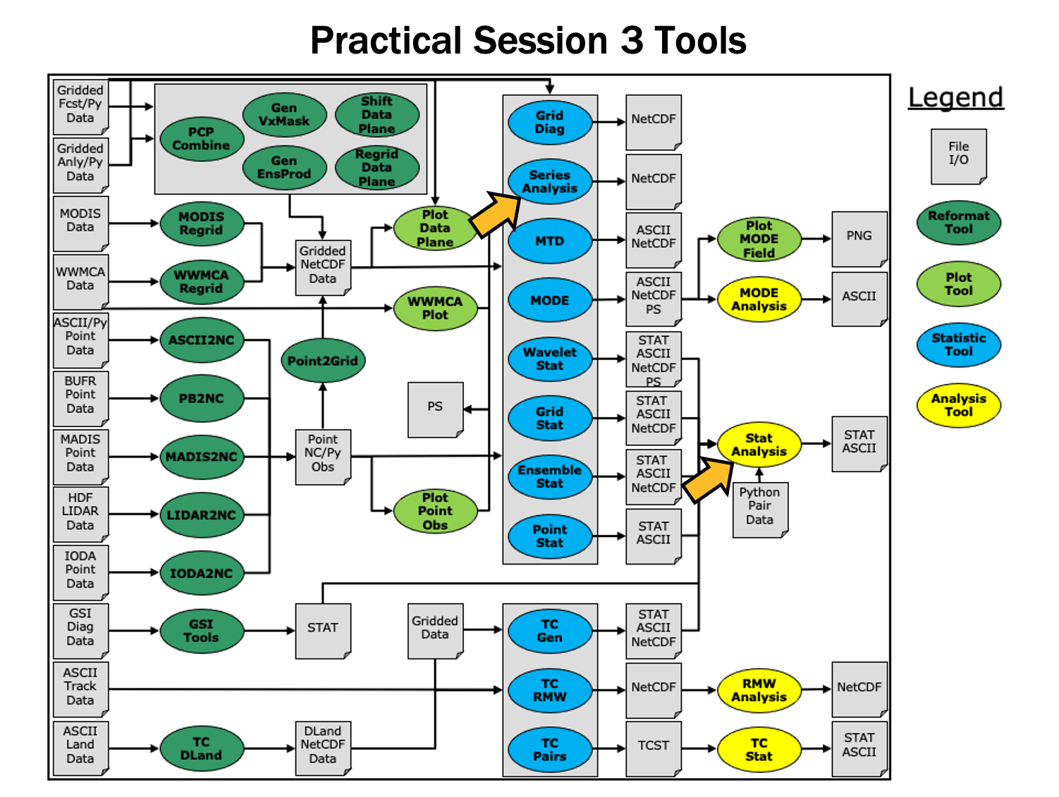 You may navigate through this tutorial by following the links at the bottom of each page or by using the menu navigation.
Since you already set up your runtime enviroment in Session 1, you should be ready to go! To be sure, run through the following instructions to check that your environment is set correctly.
Prerequisites: Verify Environment is Set Correctly
Before running the tutorial instructions, you will need to ensure that you have a few environment variables set up correctly. If they are not set correctly, the tutorial instructions will not work properly.
EDIT AFTER COPYING and BEFORE HITTING RETURN!
source METplus-5.0.0_TutorialSetup.sh
echo ${METPLUS_BUILD_BASE}
echo ${MET_BUILD_BASE}
echo ${METPLUS_DATA}
ls ${METPLUS_TUTORIAL_DIR}
ls ${METPLUS_BUILD_BASE}
ls ${MET_BUILD_BASE}
ls ${METPLUS_DATA}
METPLUS_BUILD_BASE is the full path to the METplus installation (/path/to/METplus-X.Y)
MET_BUILD_BASE is the full path to the MET installation (/path/to/met-X.Y)
METPLUS_DATA is the location of the sample test data directory
ls ${METPLUS_BUILD_BASE}/ush/run_metplus.py
See the instructions in Session 1 for more information.
You are now ready to move on to the next section.
MET Tool: Stat-Analysis
MET Tool: Stat-Analysis
Stat-Analysis Tool: General
Stat-Analysis Functionality
The Stat-Analysis tool reads the ASCII output files from the Point-Stat, Grid-Stat, Wavelet-Stat, and Ensemble-Stat tools. It provides a way to filter their STAT data and summarize the statistical information they contain. If you pass it the name of a directory, Stat-Analysis searches that directory recursively and reads any .stat files it finds. Alternatively, if you pass it an explicit file name, it'll read the contents of the file regardless of the suffix, enabling it to the optional _LINE_TYPE.txt files. Stat-Analysis runs one or more analysis jobs on the input data. It can be run by specifying a single analysis job on the command line or multiple analysis jobs using a configuration file. The analysis job types are summarized below:
- The filter job simply filters out lines from one or more STAT files that meet the filtering options specified.
- The summary job operates on one column of data from a single STAT line type. It produces summary information for that column of data: mean, standard deviation, min, max, and the 10th, 25th, 50th, 75th, and 90th percentiles.
- The aggregate job aggregates STAT data across multiple time steps or masking regions. For example, it can be used to sum contingency table data or partial sums across multiple lines of data. The -line_type argument specifies the line type to be summed.
- The aggregate_stat job also aggregates STAT data, like the aggregate job above, but then derives statistics from that aggregated STAT data. For example, it can be used to sum contingency table data and then write out a line of the corresponding contingency table statistics. The -line_type and -out_line_type arguments are used to specify the conversion type.
- The ss_index job computes a skill-score index, of which the GO Index (go_index) is a special case. The GO Index is a performance metric used primarily by the United States Air Force.
- The ramp job processes a time series of data and identifies rapid changes in the forecast and observation values. These forecast and observed ramp events are used populate a 2x2 contingency table from which categorical statistics are derived.
Stat-Analysis Usage
View the usage statement for Stat-Analysis by simply typing the following:
| Usage: stat_analysis | ||
| -lookin path | Space-separated list of input paths where each is a _TYPE.txt file, STAT file, or directory which should be searched recursively for STAT files. Allows the use of wildcards (required). | |
| [-out filename] | Output path or specific filename to which output should be written rather than the screen (optional). | |
| [-tmp_dir path] | Override the default temporary directory to be used (optional). | |
| [-log file] | Outputs log messages to the specified file | |
| [-v level] | Level of logging | |
| [-config config_file] | [JOB COMMAND LINE] (Note: "|" means "or") | ||
| [-config config_file] | STATAnalysis config file containing Stat-Analysis jobs to be run. | |
| [JOB COMMAND LINE] | All the arguments necessary to perform a single Stat-Analysis job. See the MET Users Guide for complete description of options. |
At a minimum, you must specify at least one directory or file in which to find STAT data (using the -lookin path command line option) and either a configuration file (using the -config config_file command line option) or a job command on the command line.
Configure
Configure
Stat-Analysis Tool: Configure
cd ${METPLUS_TUTORIAL_DIR}/output/met_output/stat_analysis
The behavior of Stat-Analysis is controlled by the contents of the configuration file or the job command passed to it on the command line. The default Stat-Analysis configuration may be found in the data/config/StatAnalysisConfig_default file.
You will see that most options are left blank, so the tool will use whatever it finds or whatever is specified in the command or job line. If you go down to the jobs[] section you will see a list of the jobs run for the test scripts.
"-job aggregate -line_type CTC -fcst_thresh >273.0 -vx_mask FULL -interp_mthd NEAREST",
"-job aggregate_stat -line_type CTC -out_line_type CTS -fcst_thresh >273.0 -vx_mask FULL -interp_mthd NEAREST"
];
The first job listed above will select out only the contingency table count lines (CTC) where the threshold applied is >273.0 over the FULL masking region. This should result in 2 lines, one for pressure levels P850-500 and one for pressure P1050-850. So this job will be aggregating contingency table counts across vertical levels.
The second job listed above will perform the same aggregation as the first. However, it'll dump out the corresponding contingency table statistics derived from the aggregated counts.
Run on Point-Stat output
Run on Point-Stat output
Stat-Analysis Tool: Run on Point-Stat output
-config STATAnalysisConfig_tutorial \
-lookin ../point_stat \
-v 2
The output for these two jobs are printed to the screen.
-config STATAnalysisConfig_tutorial \
-lookin ../point_stat \
-v 2 \
-out aggr_ctc_lines.out
The output was written to aggr_ctc_lines.out. We'll look at this file in the next section.
-lookin ../point_stat \
-v 2 \
-job aggregate \
-line_type CTC \
-fcst_thresh ">273.0" \
-vx_mask FULL \
-interp_mthd NEAREST
Note that we had to put double quotes (") around the forecast theshold string for this to work.
-lookin ../point_stat \
-v 2 \
-job aggregate \
-line_type CTC \
-fcst_thresh ">273.0" \
-vx_mask FULL \
-interp_mthd NEAREST \
-dump_row aggr_ctc_job.stat \
-out_stat aggr_ctc_job_out.stat
Output
Output
Stat-Analysis Tool: Output
On the previous page, we generated the output file aggr_ctc_lines.out by using the -out command line argument.
This file contains the output for the two jobs we ran through the configuration file. The output for each job consists of 3 lines as follows:
- The JOB_LIST line contains the job filtering parameters applied for this job.
- The COL_NAME line contains the column names for the data to follow in the next line.
- The third line consists of the line type generated (CTC and CTS in this case) followed by the values computed for that line type.
-lookin ../point_stat/point_stat_run2_360000L_20070331_120000V.stat \
-v 2 \
-job aggregate \
-fcst_var TMP \
-fcst_lev Z2 \
-vx_mask EAST -vx_mask WEST \
-interp_pnts 1 \
-line_type CTC \
-fcst_thresh ">278.0"
This job should aggregate 2 CTC lines for 2-meter temperature across the EAST and WEST regions.
-
Do the same aggregation as above but for the 5x5 interpolation output (i.e. 25 points instead of 1 point).
-
Do the aggregation listed in (1) but compute the corresponding contingency table statistics (CTS) line. Hint: you will need to change the job type to aggregate_stat and specify the desired -out_line_type.
How do the scores change when you increase the number of interpolation points? Did you expect this? -
Aggregate the scalar partial sums lines (SL1L2) for 2-meter temperature across the EAST and WEST masking regions.
How does aggregating the East and West domains affect the output? -
Do the aggregation listed in (3) but compute the corresponding continuous statistics (CNT) line. Hint: use the aggregate_stat job type.
-
Run an aggregate_stat job directly on the matched pair data (MPR lines), and use the -out_line_type command line argument to select the type of output to be generated. You'll likely have to supply additional command line arguments depending on what computation you request.
- How do the scores compare to the original (separated by level) scores? What information is gained by aggregating the statistics?
Exercise Answers
Exercise Answers
- Job Number 1:
stat_analysis \
-lookin ../point_stat/point_stat_run2_360000L_20070331_120000V.stat -v 2 \
-job aggregate -fcst_var TMP -fcst_lev Z2 -vx_mask EAST -vx_mask WEST -interp_pnts 25 -fcst_thresh ">278.0" \
-line_type CTC \
-dump_row job1_ps.stat - Job Number 2:
stat_analysis \
-lookin ../point_stat/point_stat_run2_360000L_20070331_120000V.stat -v 2 \
-job aggregate_stat -fcst_var TMP -fcst_lev Z2 -vx_mask EAST -vx_mask WEST -interp_pnts 25 -fcst_thresh ">278.0" \
-line_type CTC -out_line_type CTS \
-dump_row job2_ps.stat - Job Number 3:
stat_analysis \
-lookin ../point_stat/point_stat_run2_360000L_20070331_120000V.stat -v 2 \
-job aggregate -fcst_var TMP -fcst_lev Z2 -vx_mask EAST -vx_mask WEST -interp_pnts 25 \
-line_type SL1L2 \
-dump_row job3_ps.stat - Job Number 4:
stat_analysis \
-lookin ../point_stat/point_stat_run2_360000L_20070331_120000V.stat -v 2 \
-job aggregate_stat -fcst_var TMP -fcst_lev Z2 -vx_mask EAST -vx_mask WEST -interp_pnts 25 \
-line_type SL1L2 -out_line_type CNT \
-dump_row job4_ps.stat - This MPR job recomputes contingency table statistics for 2-meter temperature over G212 using a new threshold of ">=285":
stat_analysis \
-lookin ../point_stat/point_stat_run2_360000L_20070331_120000V.stat -v 2 \
-job aggregate_stat -fcst_var TMP -fcst_lev Z2 -vx_mask G212 -interp_pnts 25 \
-line_type MPR -out_line_type CTS \
-out_fcst_thresh ge285 -out_obs_thresh ge285 \
-dump_row job5_ps.stat
METplus Use Case: StatAnalysis
METplus Use Case: StatAnalysis
The StatAnalysis use case utilizes the MET Stat-Analysis tool.
Optional: Refer to the MET Users Guide for a description of the MET tools used in this use case.
Optional: Refer to the METplus Config Glossary section of the METplus Users Guide for a reference to METplus variables used in this use case.
- Review the use case configuration file: StatAnalysis.conf
In this use-case, Stat-Analysis is performing a simple filtering job and writing the data out to a .stat file using dump_row.
Note: Several of the optional variables may be set to further stratify of the results. LOOP_LIST_ITEMS needs to have at least 1 entry for the use-case to run.
DESC_LIST =
FCST_LEAD_LIST =
OBS_LEAD_LIST =
FCST_VALID_HOUR_LIST = 12
FCST_INIT_HOUR_LIST = 00, 12
...
FCST_VAR_LIST = TMP
...
GROUP_LIST_ITEMS = FCST_INIT_HOUR_LIST
LOOP_LIST_ITEMS = FCST_VALID_HOUR_LIST, MODEL_LIST
Also note: This example uses test output from the grid_stat tool
- Run the use case:
${METPLUS_BUILD_BASE}/parm/use_cases/met_tool_wrapper/StatAnalysis/StatAnalysis.conf \
${METPLUS_TUTORIAL_DIR}/tutorial.conf \
config.OUTPUT_BASE=${METPLUS_TUTORIAL_DIR}/output/StatAnalysis
-
Review the output files:
The following output file should been generated:
You will see there are many line types, verification masks, interpolation methods, and thresholds in the filtered file. NOTE: use ":" then "set nowrap" to be able to easily see the full line
If you look at the log file in ${METPLUS_TUTORIAL_DIR}/output/StatAnalysis/logs, you will see the how the Stat-Analysis command is built and what jobs it is processing. If you want to re-run, you can copy the call to stat_analysis and the path to the -lookin file after the "COMMAND:" (excluding the -config argument) and then everything after -job after "DEBUG 2: Processing Job 1:"
OUTPUT: DEBUG 1: Default Config File: /usr/local/met-10.0.0/share/met/config/STATAnalysisConfig_default
DEBUG 1: User Config File: /usr/local/METplus-4.0.0/parm/met_config/STATAnalysisConfig_wrapped
DEBUG 2: Processing 4 STAT files.
DEBUG 2: STAT Lines read = 858
DEBUG 2: STAT Lines retained = 136
DEBUG 2:
DEBUG 2: Processing Job 1: -job filter -model WRF -fcst_valid_beg 20050807_120000 -fcst_valid_end 20050807_120000 -fcst_valid_hour 120000 -fcst_init_hour 000000 -fcst_init_hour 120000 -fcst_var TMP -obtype ANALYS -dump_row /d1/personal/jensen/tutorial/METplus-4.0.0_Tutorial/output/StatAnalysis/stat_analysis/12Z/WRF/WRF_2005080712.stat
- Copy METplus config file to aggregate statistics, and re-run
${METPLUS_TUTORIAL_DIR}/user_config/StatAnalysis_run2.conf
VX_MASK_LIST = DTC165, DTC166
OBS_THRESH_LIST = >=300,<300
LOOP_LIST_ITEMS = FCST_VALID_HOUR_LIST, MODEL_LIST, OBS_THRESH_LIST
${METPLUS_TUTORIAL_DIR}/user_config/StatAnalysis_run2.conf \
${METPLUS_TUTORIAL_DIR}/tutorial.conf \
config.OUTPUT_BASE=${METPLUS_TUTORIAL_DIR}/output/StatAnalysis_run2
- Review Directory and Log File
Which returns something that looks like the following:
Why is there no stat_analysis directory? Because we removed the -dump_row flag from the STAT_ANALYSIS_JOB_ARGS line and removed the STAT_ANALYSIS_OUTPUT_TEMPLATE value. So did anything happen? The answer is yes. There is a command line option called "-out" controlled by STAT_ANALYSIS_OUTPUT_TEMPLATE which allows a user to define the name of an output filename to capture the aggregation in a file. If the "-out" option is not set, the output is written to the screen as standard output. Let's check the log file in ${METPLUS_TUTORIAL_DIR}/output/StatAnalysis_run2/logs to see if the output is captured there.
20050807_120000 -fcst_valid_hour 120000 -fcst_init_hour 000000 -fcst_init_hour 120000 -fcst_var TMP -obtype ANALYS
-vx_mask DTC165 -vx_mask DTC166 -obs_thresh >=300 -line_type CTC -out_line_type CTS -out_alpha 0.05000
DEBUG 2: Computing output for 1 case(s).
DEBUG 2: For case "", found 2 unique VX_MASK values: DTC165,DTC166
COL_NAME: TOTAL BASER BASER_NCL BASER_NCU BASER_BCL BASER_BCU FMEAN FMEAN_NCL FMEAN_NCU FMEAN_BCL FMEAN_BCU ACC ACC_NCL ACC_NCU ACC_BCL ACC_BCU FBIAS FBIAS_BCL FBIAS_BCU PODY PODY_NCL PODY_NCU PODY_BCL PODY_BCU PODN PODN_NCL PODN_NCU PODN_BCL PODN_BCU POFD POFD_NCL POFD_NCU POFD_BCL POFD_BCU FAR FAR_NCL FAR_NCU FAR_BCL FAR_BCU CSI CSI_NCL CSI_NCU CSI_BCL CSI_BCU GSS GSS_BCL GSS_BCU HK HK_NCL HK_NCU HK_BCL HK_BCU HSS HSS_BCL HSS_BCU ODDS ODDS_NCL ODDS_NCU ODDS_BCL ODDS_BCU LODDS LODDS_NCL LODDS_NCU LODDS_BCL LODDS_BCU ORSS ORSS_NCL ORSS_NCU ORSS_BCL ORSS_BCU EDS EDS_NCL EDS_NCU EDS_BCL EDS_BCU SEDS SEDS_NCL SEDS_NCU SEDS_BCL SEDS_BCU EDI EDI_NCL EDI_NCU EDI_BCL EDI_BCU SEDI SEDI_NCL SEDI_NCU SEDI_BCL SEDI_BCU BAGSS BAGSS_BCL BAGSS_BCU CTS: 12420 0.11715 0.11161 0.12292 NA NA 0.14509 0.139 0.15139 NA NA 0.96063 0.95706 0.96391 NA NA 1.23849 NA NA 0.9512 0.94727 0.95485 NA NA 0.96188 0.95837 0.96511 NA NA 0.038121 0.034894 0.041634 NA NA 0.23196 0.22462 0.23947 NA NA 0.73892 0.73112 0.74657 NA NA 0.70576 NA NA 0.91308 0.90125 0.92491 NA NA 0.8275 NA NA 491.84743 380.09404 636.458 NA NA 6.19817 5.94042 6.45592 NA NA 0.99594 0.9949 0.99699 NA NA 0.9544 0.94404 0.96477 NA NA 0.85693 0.84708 0.86678 NA NA 0.96984 0.96086 0.97881 NA NA 0.97212 0.96147 0.9782 NA NA 0.67864 NA NA
These is the aggregate statistics computed from the summed CTC lines for the DTC165 and DTC166 masking regions for the threshold >=300. If you scroll down further, you will see the same info but for the threshold <300.
- Have output written to .stat file
${METPLUS_TUTORIAL_DIR}/user_config/StatAnalysis_run2.conf \
${METPLUS_TUTORIAL_DIR}/tutorial.conf \
config.OUTPUT_BASE=${METPLUS_TUTORIAL_DIR}/output/StatAnalysis_run3
You should see the .stat file now in the stat_analysis/12Z/WRF directory
MET Tool: Series-Analysis
MET Tool: Series-Analysis
Series-Analysis Tool: General
Series-Analysis Functionality
The Series-Analysis Tool accumulates statistics separately for each horizontal grid location over a series. Usually, the series is defined as a time series, however any type of series is possible, including a series of vertical levels. This differs from the Grid-Stat tool in that Grid-Stat computes statistics aggregated over a spatial masking region at a single point in time. The Series-Analysis Tool computes statistics for each individual grid point and can be used to quantify how the model performance varies over the domain.
Series-Analysis Usage
View the usage statement for Series-Analysis by simply typing the following:
| Usage: series_analysis | ||
| -fcst file_1 ... file_n | Gridded forecast files or ASCII file containing a list of file names. | |
| -obs file_1 ... file_n | Gridded observation files or ASCII file containing a list of file names. | |
| [-both file_1 ... file_n] | Sets the -fcst and -obs options to the same list of files (e.g. the NetCDF matched pairs files from Grid-Stat). |
|
| [-paired] | Indicates that the -fcst and -obs file lists are already matched up (i.e. the n-th forecast file matches the n-th observation file). |
|
| -out file | NetCDF output file name for the computed statistics. | |
| -config file | SeriesAnalysisConfig file containing the desired configuration settings. | |
| [-log file] | Outputs log messages to the specified file | |
| [-v level] | Level of logging (optional). | |
| [-compress level] | NetCDF compression level (optional). |
At a minimum, the -fcst, -obs (or -both), -out, and -config settings must be passed in on the command line. All forecast and observation fields must be interpolated to a common grid prior to running Series-Analysis.
Configure
Configure
Series-Analysis Tool: Configure
cd ${METPLUS_TUTORIAL_DIR}/output/met_output/series_analysis
The behavior of Series-Analysis is controlled by the contents of the configuration file passed to it on the command line. The default Series-Analysis configuration file may be found in the data/config/SeriesAnalysisConfig_default file.
The configurable items for Series-Analysis are used to specify how the verification is to be performed. The configurable items include specifications for the following:
- The forecast fields to be verified at the specified vertical level or accumulation interval.
- The threshold values to be applied.
- The area over which to limit the computation of statistics - as predefined grids or configurable lat/lon polylines.
- The confidence interval methods to be used.
- The smoothing methods to be applied.
- The types of statistics to be computed.
You may find a complete description of the configurable items in the series_analysis configuration file section of the MET User's Guide. Please take some time to review them.
-
Set the fcst dictionary to
fcst = {
field = [
{
name = "APCP";
level = [ "A3" ];
}
];
}To request the GRIB abbreviation for precipitation (APCP) accumulated over 3 hours (A3).
-
Delete obs = fcst; and insert
obs = {
field = [
{
name = "APCP_03";
level = [ "(*,*)" ];
}
];
}To request the NetCDF variable named APCP_03 where its two dimensions are the gridded dimensions (*,*).
-
Look up a few lines above the fcst dictionary and setcat_thresh = [ >0.0, >=5.0 ];
To define the categorical thresholds of interest. By defining this at the top level of config file context, these thresholds will be applied to both the fcst and obs settings.
-
In the mask dictionary, setgrid = "G212";
To limit the computation of statistics to only those grid points falling inside the NCEP Grid 212 domain.
-
Setblock_size = 10000;
To process 10,000 grid points in each pass through the data. Setting block_size larger should make the tool run faster but use more memory.
-
In the output_stats dictionary, set
fho = [ "F_RATE", "O_RATE" ];
ctc = [ "FY_OY", "FN_ON" ];
cts = [ "CSI", "GSS" ];
mctc = [];
mcts = [];
cnt = [ "TOTAL", "RMSE" ];
sl1l2 = [];
pct = [];
pstd = [];
pjc = [];
prc = [];For each line type, you can select statistics to be computed at each grid point over the series. These are the column names from those line types. Here, we select the forecast rate (FHO: F_RATE), observation rate (FHO: O_RATE), number of forecast yes and observation yes (CTC: FY_OY), number of forecast no and observation no (CTC: FN_ON), critical success index (CTS: CSI), and the Gilbert Skill Score (CTS: GSS) for each threshold, along with the root mean squared error (CNT: RMSE).
Run
Run
Series-Analysis Tool: Run
sample_obs/ST2ml_3h/sample_obs_2005080703V_03A.nc \
-pcpdir ${METPLUS_DATA}/met_test/data/sample_obs/ST2ml
sample_obs/ST2ml_3h/sample_obs_2005080706V_03A.nc \
-pcpdir ${METPLUS_DATA}/met_test/data/sample_obs/ST2ml
sample_obs/ST2ml_3h/sample_obs_2005080709V_03A.nc \
-pcpdir ${METPLUS_DATA}/met_test/data/sample_obs/ST2ml
sample_obs/ST2ml_3h/sample_obs_2005080712V_03A.nc \
-pcpdir ${METPLUS_DATA}/met_test/data/sample_obs/ST2ml
sample_obs/ST2ml_3h/sample_obs_2005080715V_03A.nc \
-pcpdir ${METPLUS_DATA}/met_test/data/sample_obs/ST2ml
sample_obs/ST2ml_3h/sample_obs_2005080718V_03A.nc \
-pcpdir ${METPLUS_DATA}/met_test/data/sample_obs/ST2ml
sample_obs/ST2ml_3h/sample_obs_2005080721V_03A.nc \
-pcpdir ${METPLUS_DATA}/met_test/data/sample_obs/ST2ml
sample_obs/ST2ml_3h/sample_obs_2005080800V_03A.nc \
-pcpdir ${METPLUS_DATA}/met_test/data/sample_obs/ST2ml
Note that the previous set of PCP-Combine commands could easily be run by looping through times in METplus Wrappers! The MET tools are often run using METplus Wrappers rather than typing individual commands by hand. You'll learn more about automation using the METplus Wrappers throughout the tutorial.
-fcst ${METPLUS_DATA}/met_test/data/sample_fcst/2005080700/wrfprs_ruc13_03.tm00_G212 \
${METPLUS_DATA}/met_test/data/sample_fcst/2005080700/wrfprs_ruc13_06.tm00_G212 \
${METPLUS_DATA}/met_test/data/sample_fcst/2005080700/wrfprs_ruc13_09.tm00_G212 \
${METPLUS_DATA}/met_test/data/sample_fcst/2005080700/wrfprs_ruc13_12.tm00_G212 \
${METPLUS_DATA}/met_test/data/sample_fcst/2005080700/wrfprs_ruc13_15.tm00_G212 \
${METPLUS_DATA}/met_test/data/sample_fcst/2005080700/wrfprs_ruc13_18.tm00_G212 \
${METPLUS_DATA}/met_test/data/sample_fcst/2005080700/wrfprs_ruc13_21.tm00_G212 \
${METPLUS_DATA}/met_test/data/sample_fcst/2005080700/wrfprs_ruc13_24.tm00_G212 \
-obs sample_obs/ST2ml_3h/sample_obs_2005080703V_03A.nc \
sample_obs/ST2ml_3h/sample_obs_2005080706V_03A.nc \
sample_obs/ST2ml_3h/sample_obs_2005080709V_03A.nc \
sample_obs/ST2ml_3h/sample_obs_2005080712V_03A.nc \
sample_obs/ST2ml_3h/sample_obs_2005080715V_03A.nc \
sample_obs/ST2ml_3h/sample_obs_2005080718V_03A.nc \
sample_obs/ST2ml_3h/sample_obs_2005080721V_03A.nc \
sample_obs/ST2ml_3h/sample_obs_2005080800V_03A.nc \
-out series_analysis_2005080700_2005080800_3A.nc \
-config SeriesAnalysisConfig_tutorial \
-v 2
The statistics we requested in the configuration file will be computed separately for each grid location and accumulated over a time series of eight three-hour accumulations over a 24-hour period. Each grid point will have up to 8 matched pair values.
Note how long this command line is. Imagine how long it would be for a series of 100 files! Instead of listing all of the input files on the command line, you can list them in an ASCII file and pass that to Series-Analysis using the -fcst and -obs options.
Output
Output
Series-Analysis Tool: Output
The output of Series-Analysis is one NetCDF file containing the requested output statistics for each grid location on the same grid as the input files.
You may view the output NetCDF file that Series-Analysis wrote using the ncdump utility. Run the following command to view the header of the NetCDF output file:
In the NetCDF header, we see that the file contains many arrays of data. For each threshold (>0.0 and >=5.0), there are values for the requested statistics: F_RATE, O_RATE, FY_OY, FN_ON, CSI, and GSS. The file also contains the requested RMSE and TOTAL number of matched pairs for each grid location over the 24-hour period.
Next, run the ncview utility to display the contents of the NetCDF output file:
Click through the different variables to see how the performance varies over the domain. Looking at the series_cnt_RMSEvariable, are the errors larger in the south eastern or north western regions of the United States?
Why does the extent of missing data increase for CSI for the higher threshold? Compare series_cts_CSI_gt0.0 to series_cts_CSI_ge5.0. (Hint: Find the definition of Critical Success index (CSI) in the MET User's Guide and look closely at the denominator.)
Try running Plot-Data-Plane to visualize the observation rate variable for non-zero precipitation (i.e. series_fho_O_RATE_gt0.0). Since the valid range of values for this data is 0 to 1, use that to set the -plot_range option.
Setting block_size to 10000 still required 3 passes through our 185x129 grid (= 23865 grid points). What happens when you increase block_size to 24000 and re-run? Does it run slower or faster?
METplus Use Case: SeriesAnalysis
METplus Use Case: SeriesAnalysis
The SeriesAnalysis use case utilizes the MET Series-Analysis tool.
Optional: Refer to the MET Users Guide for a description of the MET tools used in this use case.
Optional: Refer to the METplus Config Glossary section of the METplus Users Guide for a reference to METplus variables used in this use case.
-
Review the use case configuration file: SeriesAnalysis.conf
This use-case shows a simple example of running Series-Analysis across precipitation forecast fields at 3 different lead times. Forecast data is from WRF output, while observational data is Stage II quantitative precipitation estimates.
Note: Forecast and observation variables are referred to individually including reference to both the NAMES and LEVELS, which relate to .
FCST_VAR1_NAME = APCP
FCST_VAR1_LEVELS = A03
OBS_VAR1_NAME = APCP_03
OBS_VAR1_LEVELS = "(*,*)"
Which relates to the following fields in the MET configuration file
field = [
{
name = "APCP";
level = [ "A03" ];
}
];
}
obs = {
field = [
{
name = "APCP_03";
level = [ "(*,*)" ];
}
];
}
Also note: Paths in SeriesAnalysis.conf may reference other config options defined in a different configuration files. For example:
where INPUT_BASE which is set in the tutorial.conf configuration file. METplus config variables can reference other config variables even if they are defined in a config file that is read afterwards.
-
Run the use case:
${METPLUS_BUILD_BASE}/parm/use_cases/met_tool_wrapper/SeriesAnalysis/SeriesAnalysis.conf \
${METPLUS_TUTORIAL_DIR}/tutorial.conf \
config.OUTPUT_BASE=${METPLUS_TUTORIAL_DIR}/output/SeriesAnalysis
METplus is finished running when control returns to your terminal console and you see the following text:
-
Review the output files:
You should have output file in the following directories:
2005080700_sa.nc
netcdf \2005080700_sa {
dimensions:
lat = 129 ;
lon = 185 ;
variables:
float lat(lat, lon) ;
lat:long_name = "latitude" ;
lat:units = "degrees_north" ;
lat:standard_name = "latitude" ;
float lon(lat, lon) ;
lon:long_name = "longitude" ;
lon:units = "degrees_east" ;
lon:standard_name = "longitude" ;
int n_series ;
n_series:long_name = "length of series" ;
float series_cnt_TOTAL(lat, lon) ;
series_cnt_TOTAL:_FillValue = -9999.f ;
series_cnt_TOTAL:name = "TOTAL" ;
series_cnt_TOTAL:long_name = "Total number of matched pairs" ;
series_cnt_TOTAL:fcst_thresh = "NA" ;
series_cnt_TOTAL:obs_thresh = "NA" ;
float series_cnt_RMSE(lat, lon) ;
series_cnt_RMSE:_FillValue = -9999.f ;
series_cnt_RMSE:name = "RMSE" ;
series_cnt_RMSE:long_name = "Root mean squared error" ;
series_cnt_RMSE:fcst_thresh = "NA" ;
series_cnt_RMSE:obs_thresh = "NA" ;
float series_cnt_FBAR(lat, lon) ;
series_cnt_FBAR:_FillValue = -9999.f ;
series_cnt_FBAR:name = "FBAR" ;
series_cnt_FBAR:long_name = "Forecast mean" ;
series_cnt_FBAR:fcst_thresh = "NA" ;
series_cnt_FBAR:obs_thresh = "NA" ;
float series_cnt_OBAR(lat, lon) ;
series_cnt_OBAR:_FillValue = -9999.f ;
series_cnt_OBAR:name = "OBAR" ;
series_cnt_OBAR:long_name = "Observation mean" ;
series_cnt_OBAR:fcst_thresh = "NA" ;
series_cnt_OBAR:obs_thresh = "NA" ;
From this output, we can see CNT line type statistics: TOTAL, RMSE, FBAR, and OBAR. These correspond to what we requested from the configuration file for output:
From the GUI that pops up, select the series_cnt_RMSE variable to view it. The image that displays is the RMSE value calculated at each grid point across the three lead times selected in the METplus configuration file.
There are two more files located in the output directory that while not statistically useful, do contain information on how METplus ran the SeriesAnalysis configuration file.
FCST_FILES contains all of the files that were found fitting the input templates for the forecast files. These are controlled by FCST_SERIES_ANALYSIS_INPUT_DIR and FCST_SERIES_ANALYSIS_INPUT_TEMPLATE. In our configuration file, these are set to
FCST_SERIES_ANALYSIS_INPUT_TEMPLATE = {init?fmt=%Y%m%d%H}/wrfprs_ruc13_{lead?fmt=%2H}.tm00_G212
Because {INPUT_BASE} is not changing for this run and the use case uses one initialization time, the lead sequences, set with the LEAD_SEQ variable and substituted in for {lead?fmt=%2H} in FCST_SERIES_ANALYSIS_INPUT_TEMPLATE, are what causes multiple files to be found. Specifically, FCST_FILES has three listed files, matching the LEAD_SEQ list from the configuration file.
Likewise, OBS_FILES contains all of the files that were found fitting the input templates for the observation files. These were controlled by OBS_SERIES_ANALYSIS_INPUT_DIR and OBS_SERIES_ANALYSIS_INPUT_TEMPLATE found in the configuration file.
-
Review the log output:
Log files for this run are found in ${METPLUS_TUTORIAL_DIR}/output/SeriesAnalysis/logs. The filename contains a timestamp of the current day.
Inside the log file all of the configuration options are listed, as well as the command that was used to call Series-Analysis:
Note that FCST_FILES and OBS_FILES were passed at runtime, rather than individual files.
There's also room for improvement noted in the low level verbosity comments of the log file:
WARNING:
WARNING: A block size of 1024 for a 185 x 129 grid requires 24 passes through the data which will be slow.
WARNING: Consider increasing "block_size" in the configuration file based on available memory.
WARNING:
This is a result of not setting the SERIES_ANALYSIS_BLOCK_SIZE in the METplus configuration file, which then defaults to the MET_INSTALL_DIR/share/met/config/SeriesAnalysisConfig_default value of 1024.
-
Create imagery for a variable in the netCDF output
While ncview was used to review the statistical imagery created by SeriesAnalysis, there is always the option to create an image using the Plot-Data-Plane tool. These images can be easily shared with others and used to demonstrate output in a presentation.
Use the following command to generate an image of the RMSE:
${METPLUS_TUTORIAL_DIR}/output/SeriesAnalysis/met_tool_wrapper/SeriesAnalysis/2005080700_sa.nc \
${METPLUS_TUTORIAL_DIR}/output/SeriesAnalysis/met_tool_wrapper/SeriesAnalysis/2005080700_RMSE.ps \
'name="series_cnt_RMSE"; level="(*,*)";'
The successful run of that command should produce an image. view it with the following command:
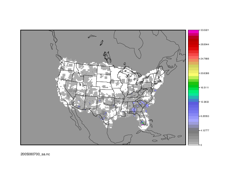
End of Session 3
End of Session 3
End of Session 3
Congratulations! You have completed Session 3!
Session 4: Ensemble and PQPF
Session 4: Ensemble and PQPF
METplus Practical Session 4
During this practical session, you will run the tools indicated below:
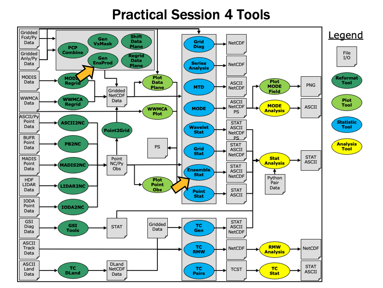
Since you already set up your runtime enviroment in Session 1, you should be ready to go! To be sure, run through the following instructions to check that your environment is set correctly.
Prerequisites: Verify Environment is Set Correctly
Before running the tutorial instructions, you will need to ensure that you have a few environment variables set up correctly. If they are not set correctly, the tutorial instructions will not work properly.
EDIT AFTER COPYING and BEFORE HITTING RETURN!
source METplus-5.0.0_TutorialSetup.sh
echo ${METPLUS_BUILD_BASE}
echo ${MET_BUILD_BASE}
echo ${METPLUS_DATA}
ls ${METPLUS_TUTORIAL_DIR}
ls ${METPLUS_BUILD_BASE}
ls ${MET_BUILD_BASE}
ls ${METPLUS_DATA}
METPLUS_BUILD_BASE is the full path to the METplus installation (/path/to/METplus-X.Y)
MET_BUILD_BASE is the full path to the MET installation (/path/to/met-X.Y)
METPLUS_DATA is the location of the sample test data directory
ls ${METPLUS_BUILD_BASE}/ush/run_metplus.py
See the instructions in Session 1 for more information.
You are now ready to move on to the next section.
MET Tool: Gen-Ens-Prod
MET Tool: Gen-Ens-Prod
Gen-Ens-Prod Tool: General
Gen-Ens-Prod Functionality
The Gen-Ens-Prod tool may be used to generate simple ensemble products from the provided ensemble forecast members. If climatological mean and standard deviation data is provided, it can be used to set thresholds for the ensemble product generation at each grid point. This tool does not provide methods to generate statistical output from the ensemble members, nor does it allow comparisons. If this is the desired outcome, Gen-Ens-Prod output can be passed to additional MET tools for further verification steps.
Gen-Ens-Prod Usage
View the usage statement for Gen-Ens-Prod by simply typing the following:
| Usage: gen_ens_prod | ||
| -ens file_1 ... file_n | ens_file_list | Input gridded ensemble files to be used, or ASCII list of ensemble member file names. | |
| -out file | netCDF output file. | |
| -config file | GenEnsProd file containing the desired configuration settings. | |
| [-ctrl file] | Contains the ensemble control data (optional). | |
| [-log file] | Outputs log messages to the specified file (optional). | |
| [-v level] | Level of logging (optional). |
Gen-Ens-Prod has three required arguments. You can specify the list of ensemble files to be used either by entering the file name for each ensemble member file (-ens ens_file_1 ... ens_file_n) or as an ASCII file containing the names of the ensemble files to be used (ens_file_list). Choose whichever way is most convenient for you. The output netCDF file containing the requested ensemble products is set with -out file. Finally, -config file requires a configuration file for processing.
Gen-Ens-Prod has additional optional settings. These include the -ctrl file, allowing users to set an ensemble control member file. This file's data will be included for ensemble mean computations, but excluded for ensemble spread. Log messages created during runtime can be saved using -log file. And as seen in other MET tools, -v level will control the verbosity of the tool's log messages.
Configure
Configure
cd ${METPLUS_TUTORIAL_DIR}/output/met_output/gen_ens_prod
Similar to other MET tools, the behavior of Gen-Ens-Prod is controlled by the contents of the configuration file passed to it on the command line. The default Gen-Ens-Prod configuration file may be found in the data/config/GenEnsProdConfig_default file. The configurations used by the test script may be found in the scripts/config/GenEnsProdConfig* files.
The configurable items for Gen-Ens-Prod are a more limited version of those found in tools such as Grid-Stat and Point-Stat. The reason for this is tied to the purpose of the tool: Gen-Ens-Prod is for creating simple ensemble products and not for statistical verification with observation datasets. This is made clear in the configuration file's use of the ensemble ens dictionary, rather than a forecast and observation dictionary.
ens_thresh = 1.0;
vld_thresh = 1.0;
field = [
{
name = "APCP";
level = "A03";
cat_thresh = [ >0.0, >=5.0 ];
}
];
}
The configuration file also does not have the ability to request statistical line type output, instead allowing users to create ensemble products with the ensemble_flag dictionary.
latlon = TRUE;
mean = TRUE;
stdev = TRUE;
minus = TRUE;
plus = TRUE;
min = TRUE;
max = TRUE;
range = TRUE;
vld_count = TRUE;
frequency = TRUE;
nep = FALSE;
nmep = FALSE;
climo = FALSE;
climo_cdp = FALSE;
}
For this tutorial, we'll configure Ensemble-Stat to verify 24-hour accumulated precipitation. While we'll run Ensemble-Stat on a single field, please note that it may be configured to operate on multiple fields. The ensemble we're verifying consists of 6 members defined over the west coast of the United States.
ens_thresh = 0.5;
vld_thresh = 0.5;
field = [
{
name = "APCP";
level = "A24";
cat_thresh = [ >0.0, >=13.0, >=25.0, >=101.0];
}
];
}
Setting ens_thresh at 0.5 allows half of the ensemble member files being passed at runtime to contain invalid data and before GenEnsProd quits with an error. Similarly, vld_thresh at 0.5 allows each grid point to have invalid data for half of the ensemble member files passed at runtime and still compute the requested products for that grid point.
latlon = TRUE;
mean = TRUE;
stdev = TRUE;
minus = FALSE;
plus = FALSE;
min = FALSE;
max = FALSE;
range = FALSE;
vld_count = TRUE;
frequency = TRUE;
nep = FALSE;
nmep = FALSE;
climo = FALSE;
climo_cdp = FALSE;
}
These products will be output to the netCDF designated at runtime with the -out flag. They will show a small sample of the options from Gen-Ens-Prod, as well as highlighting how the output changes when one of the files is entered as the control ensemble member, which will be done later this session.
Run
Run
-ens ${METPLUS_DATA}/met_test/data/sample_fcst/2009123112/*gep*/d01_2009123112_02400.grib \
-out ./GenEnsProd_APCP24.nc \
-config GenEnsProdConfig_tutorial \
-v 2
Gen-Ens-Prod creates the products we requested in the configuration file, using the categorical thresholds specified. Note that we've passed the input ensemble data directly on the command line by specifying the ensemble member names using wildcards.
When Gen-Ens-Prod has completed running, there will be 1 netCDF output file, GenEnsProd_APCP24.nc
(content)
Output
Output
As mentioned previously, Gen-Ens-Prod only produces 1 netCDF output file. This file contains all of the requested products that were made in the configuration file.
Note that the file contains 9 variables: the latitude and longitudes, the ensemble mean and standard deviation, the ensemble valid data count, and the four categorical thresholds that were set, all with the prefix APCP_24_A24_ENS_FREQ_. These thresholds act as uncalibrated probability forecasts and can be verified against observational datasets with other MET tools.
Click through the variable names in the ncview window to see plots of the content we saw in the ncdump command.
Now that we've seen a successful run of the Gen-Ens-Prod tool, let's change the run command slightly to show how the -ctrl setting works.
Rerun
Rerun
Now that we've seen the output for Gen-Ens-Prod without any control ensemble members, let's change the run slightly by selecting one of the previous ensemble members as the control. Because the required changes will be performed in the run command, no edits will be made to the configuration file.
-ens ${METPLUS_DATA}/met_test/data/sample_fcst/2009123112/*gep[23567]/d01_2009123112_02400.grib \
-out ./GenEnsProd_APCP24_run2_ctrl.nc \
-config GenEnsProdConfig_tutorial \
-ctrl ${METPLUS_DATA}/met_test/data/sample_fcst/2009123112/arw-fer-gep1/d01_2009123112_02400.grib \
-v 2
When MET has successfully finished running, 1 new netCDF file will be in the current directory containing the same ensemble products that were available in the first run. However, the output is now changed by using one of the original ensemble members as the control member.
You'll see as you click through the variables that the only difference between the two runs of Gen-Ens-Prod is APCP_24_A24_ENS_STDEV. The mean (APCP_24_A24_ENS_MEAN) and all of the categorical thresholds still use all 6 ensemble members. This is quickly confirmed by viewing APCP_24_A24_ENS_VLD for both, which shows 6 ensembles were used for both runs across the domain.
To better illustrate the difference in the APCP_24_A24_ENS_STDEV products, let's calculate the difference of the two fields using PCP-Combine, and plot the results using Plot-Data-Plane.
GenEnsProd_APCP24.nc 'name="APCP_24_A24_ENS_STDEV"; level="(*,*)";' \
GenEnsProd_APCP24_run2_ctrl.nc 'name="APCP_24_A24_ENS_STDEV"; level="(*,*)";' \
Full_Ensemble_STDDEV_minus_ctrl_STDDEV.nc -name STDDEV_DIFF
'name="STDDEV_DIFF"; level="(*,*)";'
If the differences weren't apparent before, this plot makes it very clear how using a control ensemble member can drastically change a product. As long as it's desired, the -ctrl option is a quick way to run Gen-Ens-Prod without control members for some products, while including it in others.
MET Tool: Ensemble-Stat
MET Tool: Ensemble-Stat
Ensemble-Stat Tool: General
Ensemble-Stat Functionality
The Ensemble-Stat tool may be used to verify the deterministic ensemble members against gridded and/or point observations. Statistics are then derived using those observations, such as rank histograms, probability integral transform histograms, spread/skill variance, relative position and continuous ranked probability score.
Ensemble-Stat Usage
View the usage statement for Ensemble-Stat by simply typing the following:
At a minimum, the input gridded ensemble files and the configuration config_file must be passed in on the command line. You can specify the list of ensemble files to be used either as a count of the number of ensemble members followed by the file name for each (n_ens ens_fil e_1 ... ens_file_n) or as an ASCII file containing the names of the ensemble files to be used (ens_file_list). Choose whichever way is most convenient for you. The optional -grid_obs and -point_obs command line options may be used to specify gridded and/or point observations to be used for computing rank histograms and other ensemble statistics.
As with the other MET statistics tools, all ensemble data and gridded verifying observations must be interpolated to a common grid prior to processing. This may be done using the automated regrid feature in the Ensemble-Stat configuration file or by running copygb and/or wgrib2 first.
Configure
Configure
cd ${METPLUS_TUTORIAL_DIR}/output/met_output/ensemble_stat
The behavior of Ensemble-Stat is controlled by the contents of the configuration file passed to it on the command line. The default Ensemble-Stat configuration file may be found in the data/config/EnsembleStatConfig_default file. The configurations used by the test script may be found in the scripts/config/EnsembleStatConfig* files.
The configurable items for Ensemble-Stat are similar to those found in Grid-Stat and Point-Stat: forecast and observation dictionaries read in the the ensemble and observation fields, respectively, while the remaining dictionaries and options control the computed statistics and the area over which those statistics are calculated.
For this tutorial, we'll configure Ensemble-Stat to verify 24-hour accumulated precipitation. While we'll run Ensemble-Stat on a single field, please note that it may be configured to operate on multiple fields. The ensemble we're verifying consists of 6 members defined over the west coast of the United States.
-
In the fcst dictionary, setfield = [
{
name = "APCP";
level = [ "A24" ];
}
];To verify the 24-hour accumulated precipitation fields.
-
In the observation filtering options, set:message_type = [ "ADPSFC" ];
To verify against surface observations.
-
In the field entry section, set:prob_cat_thresh= [ >=0, >=5.0, >=10.0 ];
To specify thresholds to use for computation of the Ranked Probability Score (RPS).
-
In the mask dictionary, setpoly = [ "MET_BASE/poly/NWC.poly",
"MET_BASE/poly/SWC.poly" ];To also verify over the northwest coast (NWC) and southwest coast (SWC) subregions.
-
Set:output_flag = {
ecnt = BOTH;
rhist = BOTH;
phist = BOTH;
orank = BOTH;
ssvar = BOTH;
relp = BOTH;
}To compute continuous ensemble statistics (ECNT), ranked histogram (RHIST), probability integral transform histogram (PHIST), observation ranks (ORANK), spread-skill variance (SSVAR), and relative position (RELP).
Run
Run
6 ${METPLUS_DATA}/met_test/data/sample_fcst/2009123112/*gep*/d01_2009123112_02400.grib \
EnsembleStatConfig_tutorial \
-grid_obs ${METPLUS_DATA}/met_test/data/sample_obs/ST4/ST4.2010010112.24h \
-point_obs ${METPLUS_DATA}/met_test/out/ascii2nc/precip24_2010010112.nc \
-outdir . \
-v 2
Ensemble-Stat is now performing the tasks we requested in the configuration file. Note that we've passed the input ensemble data directly on the command line by specifying the number of ensemble members (6) followed by their names using wildcards. We've also specified one gridded StageIV analysis field (-grid_obs) and one file containing point rain gauge observations (-point_obs) to be used in computing rank histograms. This tool should run pretty quickly.
When Ensemble-Stat is finished, it will have created 8 output files in the current directory: 7 ASCII statistics files (.stat, _ecnt.txt, _rhist.txt, _phist.txt, _orank.txt, _ssvar.txt , and _relp.txt ), and a NetCDF matched pairs file (_orank.nc).
Output
Output
The output from Ensemble-Stat is one or more ASCII files containing statistics summarizing the verification performed, and a NetCDF file containing the gridded matched pairs.
All of the line types are written to the file ending in .stat. The Ensemble-Stat tool currently writes 12 output line types: ECNT, RPS, RHIST, PHIST, RELP, SSVAR, PCT, PSTD, PJC, PRC, ECLV, and ORANK.
- The ECNT line type contains contains continuous ensemble statistics such as spread and skill. Ensemble-Stat uses assumed observation errors to compute both perturbed and unperturbed versions of these statistics. Statistics to which observation error have been applied can be found in columns which include the _OERR (for observation error) suffix.
- The RPS line type contains the Ranked Probability Score, as well as the number of ensembles that were used to calculate the score, the Ranked Probability Skill Score, and the Ranked Probability Score decomposed into its terms of reliability, resolution, and uncertainty.
- The RHIST line type contains counts for a ranked histogram. This ranks each observation value relative to ensemble member values. Ideally, observation values would fall equally across all available ranks, yielding a flat rank histogram. In practice, ensembles are often under-(U shape) or over-(inverted U shape) dispersive. In the event of ties, ranks are randomly assigned.
- The PHIST line type contains counts for a probability integral transform histogram. This scales the observation ranks to a range of values between 0 and 1 and allows ensembles of different size to be compared. Similarly, when ensemble members drop out, RHIST lines cannot be aggregated together but PHIST lines can.
- The RELP line is the relative position, which indicates how often each ensemble member's value was closest to the observation's value. In the event of ties, credit is divided equally among the tied members.
- The PCT line type contains the contingency table counts for probabilistic forecasts.
- The PSTD line type is the probabilistic statistics for dichotomous outcomes for derived ensemble relative frequencies.
- The PJC line type contains joint and conditional factorization for derived ensemble relative frequencies
- The PRC line type has the receiver operating characteristic for derived ensemble relative frequencies
- The ECLV line type is the economic cost/loss relative value for derived ensemble relative frequencies
- The ORANK line type is similar to the matched pair (MPR) output of Point-Stat. For each point observation value, one ORANK line is written out containing the observation value, its rank, and the corresponding ensemble values for that point. When verifying against a griddedanalysis, the ranks can be written to the NetCDF output file.
- The SSVAR line contains binned spread/skill information. For each observation location, the ensemble variance is computed at that point. Those variance values are binned based on the ens_ssvar_bin_size configuration setting. The skill is determined by comparing the ensemble mean value to the observation value. One SSVAR line is written for each bin summarizing the all the observation/ensemble mean pairs that it contains.
The STAT file contains all the ASCII output while the _ecnt.txt, _rhist.txt, _phist.txt, _orank.txt, _ssvar.txt, and _relp.txt files contain the same data but sorted by line type. Since so much data can be written for the ORANK line type, we recommend disabling the output of the optional text file using the output_flag parameter in the configuration file.
- There are 6 lines in this output file resulting from using 3 verification regions in the VX_MASK column (FULL, NWC, and SWC) and two observations datasets in the OBTYPE column (ADPSFC point observations and gridded observations).
- Each line contains columns for the observation ranks (RANK_#) and a handful of ensemble statistics (CRPS, CRPSS, IGN, and SPREAD).
- There is output for 7 ranks - since we verified a 6-member ensemble, there are 7 possible ranks the observation values could attain.
- There are 5 lines in this output file resulting from using 3 verification regions (FULL, NWC, and SWC) and two observations datasets (ADPSFC point observations and gridded observations), where the ADPSFC point observations for the SWC region were all zeros for which the probability integral transform is not defined.
- Each line contains columns for the BIN_SIZE and counts for each bin. The bin size is set in the configuration file using the ens_phist_bin_size field. In this case, it was set to .05, therefore creating 20 bins (1/ens_phist_bin_size).
- This file contains 1866 lines, 1 line for each observation value falling inside each verification region (VX_MASK).
- Each line contains 44 columns, including header information, the observation location and value, its rank, and the 6 values for the ensemble members at that point.
- When there are ties, Ensemble-Stat randomly assigns a rank from all the possible choices. This can be seen in the SWC masking region where all of the observed values are 0 and the ensemble forecasts are 0 as well. Ensemble-Stat randomly assigns a rank between 1 and 7.
This file is only created when you've verified using gridded observations and have requested its output using the output_flag parameter in the configuration file. Click through the variables in this file. Note that for each of the three verification areas (FULL, NWC, and SWC) this file contains 4 variables:
- The gridded observation value
- The observation rank
- The probability integral transform
- The ensemble valid data count
In ncview, the random assignment of tied ranks is evident in areas of zero precipitation.
Feel free to explore using this dataset. Some options to try are:
- Try setting skip_const = TRUE; in the config file to discard points where all ensemble members and the observation are tied (i.e. zero precip). If you want to save it to a different file, make sure you set output_prefix to something meaningful, such as "run2", or "skip-constant".
- Try setting obs_thresh = [ >0.01 ]; in the config file to only consider points where the observation meets this threshold. How does this differ from the using skip_const?
- Use wgrib to inventory the input files and add additional entries to the ens.field list. Can you process 10-meter U and V wind?
METplus Use Case: GenEnsProd and EnsembleStat
METplus Use Case: GenEnsProd and EnsembleStat
Both the Ensemble-Stat tool and Gen-Ens-Prod tool have METplus wrapper versions. We will review a METplus use case that calls on both of these tools and see how they interact with and compliment each other.
Optional: Refer to the METplus Config Glossary section of the METplus Users Guide for a reference to METplus variables used in this use case.
- Review the basic wrapper configuration file: EnsembleStat.conf
Recall that the Ensemble-Stat tool is for verification against gridded and/or point observation datasets and can calculate statistical output, which is reflected in the wrapper's configuration options. Note that variables in EnsembleStat.conf reference other config variables that have been defined in other configuration files. For example:
This references INPUT_BASE which is set in the tutorial.conf configuration file. METplus config variables can reference other config variables even if they are defined in a config file that is read afterwards. This is a common practice in METplus wrappers, including the use case that we'll be running.
- Review the basic wrapper configuration file: GenEnsProd.conf
The Gen-Ens-Prod tool (and its wrapper that we're now using) is for creating ensemble products. This differs from the purpose of the Ensemble-Stat tool, so the GenEnsProd wrapper options will differ from those in the EnsembleStat wrapper.
- Review the use case configuration file: EnsembleStat_fcstHRRRE_obsHRRRE_Sfc_MultiField.conf
For the use case that we will be running, three tool wrappers are called: PB2NC, GenEnsProd, and EnsembleStat. These tools will iterate over one time step, but three separate lead times. PB2NC is used as a conversion method for the input file types and was covered in a previous session. From the order of the tools in PROCESS_LIST, we see that EnsembleStat runs first. Since that tool is for verification and statistical output, it uses observational field settings like OBS_VAR1_NAME and BOTH_VAR1_THRESH, which applies to both the forecast and observation variable 1. It also will create multiple output files for each time step processed, one for each of the requested line types:
ENSEMBLE_STAT_OUTPUT_FLAG_RPS = NONE
ENSEMBLE_STAT_OUTPUT_FLAG_RHIST = BOTH
ENSEMBLE_STAT_OUTPUT_FLAG_PHIST = BOTH
ENSEMBLE_STAT_OUTPUT_FLAG_ORANK = BOTH
ENSEMBLE_STAT_OUTPUT_FLAG_SSVAR = BOTH
ENSEMBLE_STAT_OUTPUT_FLAG_RELP = BOTH
GenEnsProd, on the other hand, will utilize the ENS_ configuration settings, and will place all output for each time step into a single netCDF output. Those file's locations and names can be seen with the following configuration settings:
GEN_ENS_PROD_OUTPUT_TEMPLATE = {init?fmt=%Y%m%d%H%M}/gen_ens_prod_{ENSEMBLE_STAT_OUTPUT_PREFIX}_{valid?fmt=%Y%m%d_%H%M%S}V_ens.nc
Note that the output directory is dependent on a different configuration setting, ENSEMBLE_STAT_OUTPUT_DIR. As mentioned above, this is common practice in METplus.
-
Run the use case:
${METPLUS_BUILD_BASE}/parm/use_cases/model_applications/short_range/EnsembleStat_fcstHRRRE_obsHRRRE_Sfc_MultiField.conf \
${METPLUS_TUTORIAL_DIR}/tutorial.conf \
config.OUTPUT_BASE=${METPLUS_TUTORIAL_DIR}/output/Ensemble
METplus is finished running when control returns to your terminal console and you see the following text:
- Review the output files:
You should have output files in the following directories:
- ensemble_stat_HRRRE_F000_ADPSFC_20180709_120000V_ecnt.txt
- ensemble_stat_HRRRE_F000_ADPSFC_20180709_120000V_orank.txt
- ensemble_stat_HRRRE_F000_ADPSFC_20180709_120000V_phist.txt
- ensemble_stat_HRRRE_F000_ADPSFC_20180709_120000V_relp.txt
- ensemble_stat_HRRRE_F000_ADPSFC_20180709_120000V_rhist.txt
- ensemble_stat_HRRRE_F000_ADPSFC_20180709_120000V_ssvar.txt
- ensemble_stat_HRRRE_F000_ADPSFC_20180709_120000V.stat
- ensemble_stat_HRRRE_F001_ADPSFC_20180709_130000V_ecnt.txt
- ensemble_stat_HRRRE_F001_ADPSFC_20180709_130000V_orank.txt
- ensemble_stat_HRRRE_F001_ADPSFC_20180709_130000V_phist.txt
- ensemble_stat_HRRRE_F001_ADPSFC_20180709_130000V_relp.txt
- ensemble_stat_HRRRE_F001_ADPSFC_20180709_130000V_rhist.txt
- ensemble_stat_HRRRE_F001_ADPSFC_20180709_130000V_ssvar.txt
- ensemble_stat_HRRRE_F001_ADPSFC_20180709_130000V.stat
- ensemble_stat_HRRRE_F002_ADPSFC_20180709_140000V_ecnt.txt
- ensemble_stat_HRRRE_F002_ADPSFC_20180709_140000V_orank.txt
- ensemble_stat_HRRRE_F002_ADPSFC_20180709_140000V_phist.txt
- ensemble_stat_HRRRE_F002_ADPSFC_20180709_140000V_relp.txt
- ensemble_stat_HRRRE_F002_ADPSFC_20180709_140000V_rhist.txt
- ensemble_stat_HRRRE_F002_ADPSFC_20180709_140000V_ssvar.txt
- ensemble_stat_HRRRE_F002_ADPSFC_20180709_140000V.stat
- gen_ens_prod_HRRRE_F000_ADPSFC_20180709_120000V_ens.nc
- gen_ens_prod_HRRRE_F001_ADPSFC_20180709_130000V_ens.nc
- gen_ens_prod_HRRRE_F002_ADPSFC_20180709_140000V_ens.nc
We can tell from the name of the files, specifically the _F00x_ string, that three different lead times were run: 0, 1, and 2. These ended up as valid times of 12z, 13z, and 14z, as indicated by the 1x0000V strings.
This stat file contains all of the statistic line types that were requested in the configuration file. If we wanted to review only one line type at a time, ECNT for example, we could instead look at the ASCII file for this lead time with the _ecnt string at the end of the file name. That file exists because the use case configuration file set:
signaling that the ecnt line type results should be in the .stat file, as well as a separate ASCII file.
- Review the log output:
Log files for this run are found in ${METPLUS_TUTORIAL_DIR}/output/Ensemble/logs. The filename contains a timestamp of the day and time that the use case was run.
-
Review the Final Configuration File:
The final configuration file is called metplus_final.conf.*, where the final string is a timestamp of the day and time the use case was run, similar to the log files. This contains all of the configuration variables used in the run. If you complete a run of METplus and are unsure how the system interpreted something from the configuration file, this is a great source of information.
METplus Use Case: EnsembleStat with multiple variable and leads
METplus Use Case: EnsembleStat with multiple variable and leads
This use case takes the PB2NC tool and combines it with the Ensemble-Stat tool, analyzing multiple forecast fields and producing ensemble relative frequencies.
Optional: Refer to the METplus Config Glossary section of the METplus Users Guide for a reference to METplus variables used in this use case.
-
Review the use case configuration file: EnsembleStat_fcstHRRRE_obsHRRRE_Sfc_MultiField.conf
Open the file and look at all of the configuration variables that are defined.
Note that in this use case, the PB2NC GenEnsProd, and EnsembleStat tools will be called:
Another important aspect of this use case is its use of lead times. While INIT_BEG and INIT_END are the same, there are three leads listed:
And that controls what files are looked at in the EnsembleStat call:
{init?fmt=%Y%m%d%H}/postprd_mem0002/wrfprs_conus_mem0002_{lead?fmt=%HH}.grib2
Given the lead times and INIT time, the tools will loop over the following valid times:
-
20180709 at 12z
-
20180709 at 13z
-
20180709 at 14z
The run time for this use case is expected to be longer, due to the multiple lead times, two MET tools, and 6 variables at multiple thresholds being analyzed.
-
Run the use case:
${METPLUS_BUILD_BASE}/parm/use_cases/model_applications/short_range/EnsembleStat_fcstHRRRE_obsHRRRE_Sfc_MultiField.conf \
${METPLUS_TUTORIAL_DIR}/tutorial.conf \
config.OUTPUT_BASE=${METPLUS_TUTORIAL_DIR}/output/Ensemble
METplus is finished running when control returns to your terminal console and you see the following text:
-
Review the output files:
You should have two directories of interest:
- EnsembleStat
-
rap
These two directories correspond to the output directories for two of the tools in the configuration file:
Take a look at the output from PB2NC first:
You'll see 3 output files, corresponding to the three lead times that were run. These files were read in by the EnsembleStat call and processed for statistics. Taking a look at those files we see a lot of output:
Each lead time is responsible for producing 8 files, for a total of 24 files. These were all requested with the ENSEMBLE_STAT_OUTPUT_FLAG options, with the exception of the .stat and .nc files.
-
Compare the netCDF output to the .stat output:
To better understand the difference between the FCST and ENS entries in the configuration file used by the EnsembleStat and GenEnsProd tools respectively, take a look at the netCDF file for the first lead time (0):
You'll notice that the majority of the extensive variables listed have the words "ENS_FREQ". This is because those variables were called with the ENSEMBLE_FLAG options: GenEnsProd will provide a summary of all fields requested across the ensemble for those ENS_VAR<n> variables.
Now look at the .stat file for the same lead time:
In the VX_MASK column, the four mask files requested are listed, along with the various line types that were requested (listed in the LINE_TYPE column). What's important to note is the lack of variable variety that was present in the netCDF: in fact, the only variable listed is TMP at the Z2 level. That's because in the configuration file, only 1 variable was requested with the FCST_VAR<n> options, and only those variables will be used for verification.
METplus Use Case: PQPF
METplus Use Case: PQPF
METplus Use Case: QPF Probabilistic
The QPF Probabilistic use case utilizes the MET Pcp-Combine, Regrid-Data-Plane, and Grid-Stat tools.
Optional: Refer to the METplus Config Glossary section of the METplus Users Guide for a reference to METplus variables used in this use case.
Review Use Case Configuration File
The configuration file is located in use_cases/model_applications/precipitation and is called GridStat_fcstHRRR-TLE_obsStgIV_GRIB.conf
Note that several processes are called in this use-case and that there is a specific setting to tell METplus that the forecast field is probabilistic. For example:
FCST_IS_PROB = true
Also note that variables in GridStat_fcstHRRR-TLE_obsStgIV_GRIB.conf reference other config variables that have been defined in configuration files. For example:
OBS_PCP_COMBINE_INPUT_DIR = {INPUT_BASE}/model_applications/precipitation/StageIV
This references INPUT_BASE which is set in the METplus tutorial.conf file (${METPLUS_TUTORIAL_DIR}/tutorial.conf). METplus config variables can reference other config variables even if they are defined in a config file that is read afterwards.
Run METplus
${METPLUS_BUILD_BASE}/parm/use_cases/model_applications/precipitation/GridStat_fcstHRRR-TLE_obsStgIV_GRIB.conf \
${METPLUS_TUTORIAL_DIR}/tutorial.conf \
config.OUTPUT_BASE=${METPLUS_TUTORIAL_DIR}/output/PQPF
METplus is finished running when control returns to your terminal console and you see the following text:
Review the Output Files
You should have output files in the following directories:
- grid_stat_PROB_PHPT_APCP_vs_STAGE4_GRIB_APCP_A06_060000L_20160904_180000V_pct.txt
- grid_stat_PROB_PHPT_APCP_vs_STAGE4_GRIB_APCP_A06_060000L_20160904_180000V_pjc.txt
- grid_stat_PROB_PHPT_APCP_vs_STAGE4_GRIB_APCP_A06_060000L_20160904_180000V_prc.txt
- grid_stat_PROB_PHPT_APCP_vs_STAGE4_GRIB_APCP_A06_060000L_20160904_180000V_pstd.txt
- grid_stat_PROB_PHPT_APCP_vs_STAGE4_GRIB_APCP_A06_060000L_20160904_180000V.stat
- grid_stat_PROB_PHPT_APCP_vs_STAGE4_GRIB_APCP_A06_070000L_20160904_190000V_pct.txt
- grid_stat_PROB_PHPT_APCP_vs_STAGE4_GRIB_APCP_A06_070000L_20160904_190000V_pjc.txt
- grid_stat_PROB_PHPT_APCP_vs_STAGE4_GRIB_APCP_A06_070000L_20160904_190000V_prc.txt
- grid_stat_PROB_PHPT_APCP_vs_STAGE4_GRIB_APCP_A06_070000L_20160904_190000V_pstd.txt
- grid_stat_PROB_PHPT_APCP_vs_STAGE4_GRIB_APCP_A06_070000L_20160904_190000V.stat
Review the Log Files
Log files for this run are found in ${METPLUS_TUTORIAL_DIR}/output/PQPF/logs. The filename contains a timestamp of the year, month, day, hour, minute, second that the METplus command was run. The log file for this command will be the most recent one.
Review the Final Configuration File
The final configuration files are found in ${METPLUS_TUTORIAL_DIR}/output/PQPF. Similar to the log files, the configuration file contains a timestamp of the time that the METplus command was run.
End of Session 4 and Additional Exercises
End of Session 4 and Additional Exercises
End of Practical Session 4
Congratulations! You have completed Session 4!
If you have extra time, you may want to try these additional METplus exercises. The answers are found on the next page.
${METPLUS_TUTORIAL_DIR}/user_config/GridStat-ensemble.accum_3hr.conf
${METPLUS_TUTORIAL_DIR}/user_config/GridStat-ensemble.accum_3hr.conf \
${METPLUS_TUTORIAL_DIR}/tutorial.conf \
config.OUTPUT_BASE=${METPLUS_TUTORIAL_DIR}/output/exercises/accum_3hr
DEBUG 1: Reading data (name="APCP"; level="A01";) from input file: /d1/projects/METplus/METplus_Data/model_applications/precipitation/StageIV/20160904/ST4.2016090418.01h
DEBUG 1: Reading data (name="APCP"; level="A01";) from input file: /d1/projects/METplus/METplus_Data/model_applications/precipitation/StageIV/20160904/ST4.2016090417.01h
DEBUG 1: Reading data (name="APCP"; level="A01";) from input file: /d1/projects/METplus/METplus_Data/model_applications/precipitation/StageIV/20160904/ST4.2016090416.01h
DEBUG 2: Skipping 480079 of 987601 grid points which do not meet the valid data threshold (1).
DEBUG 1: Creating output file: /path/to/tutorial/output/exercises/accum_3hr/model_applications/precipitation/GridStat_fcstHRRR-TLE_obsStgIV_GRIB/uswrp/StageIV_grib/bucket/20160904/ST4.2016090418_A03h
DEBUG 2: Writing output variable "APCP_03" for the "sum" of "APCP/A01".
From the log output found in ${METPLUS_TUTORIAL_DIR}/output/logs:
DEBUG 1: Reading data (name="APCP"; level="A6";) from input file: /path/to/METplus_Data/qpf/uswrp/StageIV/20160904/ST4.2016090418.06h
DEBUG 2: Skipping 399779 of 987601 grid points which do not meet the valid data threshold (1).
DEBUG 1: Creating output file: /path/to/tutorial/output/qpf-prob/uswrp/StageIV_grib/bucket/20160904/ST4.2016090418_A06h
DEBUG 2: Writing output variable "APCP_06" for the "sum" of "APCP/A6".
cp GridStat-ensemble.accum_3hr.conf GridStat-ensemble.input_1hr.conf
${METPLUS_TUTORIAL_DIR}/user_config/GridStat-ensemble.input_1hr.conf \
${METPLUS_TUTORIAL_DIR}/tutorial.conf \
config.OUTPUT_BASE=${METPLUS_TUTORIAL_DIR}/output/exercises/input_1hr
DEBUG 2: Performing derivation command (sum) for 6 files.
DEBUG 1: Reading data (name="APCP"; level="A01";) from input file: /d1/projects/METplus/METplus_Data/model_applications/precipitation/StageIV/20160904/ST4.2016090418.01h
DEBUG 1: Reading data (name="APCP"; level="A01";) from input file: /d1/projects/METplus/METplus_Data/model_applications/precipitation/StageIV/20160904/ST4.2016090417.01h
DEBUG 1: Reading data (name="APCP"; level="A01";) from input file: /d1/projects/METplus/METplus_Data/model_applications/precipitation/StageIV/20160904/ST4.2016090416.01h
DEBUG 1: Reading data (name="APCP"; level="A01";) from input file: /d1/projects/METplus/METplus_Data/model_applications/precipitation/StageIV/20160904/ST4.2016090415.01h
DEBUG 1: Reading data (name="APCP"; level="A01";) from input file: /d1/projects/METplus/METplus_Data/model_applications/precipitation/StageIV/20160904/ST4.2016090414.01h
DEBUG 1: Reading data (name="APCP"; level="A01";) from input file: /d1/projects/METplus/METplus_Data/model_applications/precipitation/StageIV/20160904/ST4.2016090413.01h
DEBUG 2: Skipping 480079 of 987601 grid points which do not meet the valid data threshold (1).
DEBUG 1: Creating output file: /path/to/tutorial/output/exercises/input_1hr/model_applications/precipitation/GridStat_fcstHRRR-TLE_obsStgIV_GRIB/uswrp/StageIV_grib/bucket/20160904/ST4.2016090418_A06h
DEBUG 2: Writing output variable "APCP_06" for the "sum" of "APCP/A01".
Answers to Exercises from Session 4
Answers to Exercises from Session 4
Answers to Exercises from Session 4
These are the answers to the exercises from the previous page. Feel free to ask a METplus team member if you have any questions!
Instructions: Modify the METplus configuration files to build a 3 hour accumulation instead of a 6 hour accumulation from forecast data using Pcp-Combine in the HREF MEAN vs. MRMS QPE example. Then compare 3 hour accumulations in the forecast and observation data with grid_stat.
Answer: In the user_config/GridStat-ensemble.accum_3hr.conf file, change the following variables in the [config] section:
Change:
To:
Instructions: Modify the METplus configuration files to force Pcp-Combine to use six 1 hour accumulation files instead of one 6 hour accumulation file of observation data in the PHPT vs. StageIV GRIB example.
Answer: In the user_config/GridStat-ensemble.input_1hr.conf file, change the following variable to the [config] section:
Change:
Back to:
Also change:
To:
Session 5: MODE and MTD
Session 5: MODE and MTD
METplus Practical Session 5
During this practical session, you will run the tools indicated below:
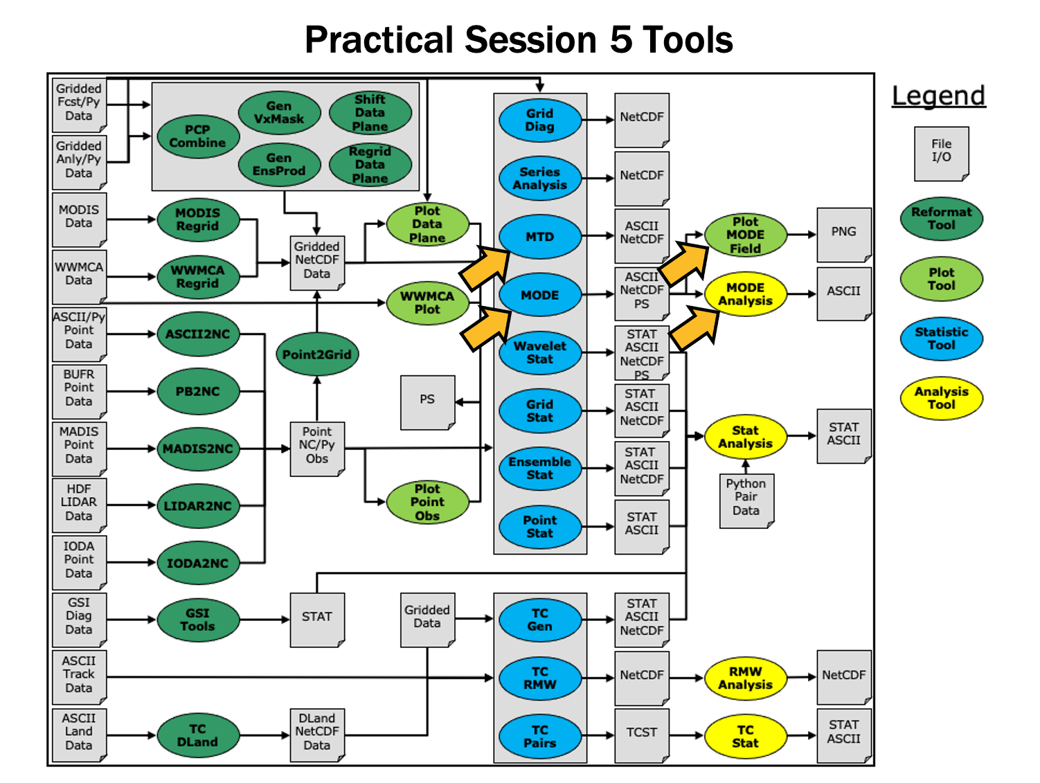
Since you already set up your runtime enviroment in Session 1, you should be ready to go! To be sure, run through the following instructions to check that your environment is set correctly.
Prerequisites: Verify Environment is Set Correctly
Before running the tutorial instructions, you will need to ensure that you have a few environment variables set up correctly. If they are not set correctly, the tutorial instructions will not work properly.
EDIT AFTER COPYING and BEFORE HITTING RETURN!
source METplus-5.0.0_TutorialSetup.sh
echo ${METPLUS_BUILD_BASE}
echo ${MET_BUILD_BASE}
echo ${METPLUS_DATA}
ls ${METPLUS_TUTORIAL_DIR}
ls ${METPLUS_BUILD_BASE}
ls ${MET_BUILD_BASE}
ls ${METPLUS_DATA}
METPLUS_BUILD_BASE is the full path to the METplus installation (/path/to/METplus-X.Y)
MET_BUILD_BASE is the full path to the MET installation (/path/to/met-X.Y)
METPLUS_DATA is the location of the sample test data directory
ls ${METPLUS_BUILD_BASE}/ush/run_metplus.py
See the instructions in Session 1 for more information.
You are now ready to move on to the next section.
MET Tool: MODE
MET Tool: MODE
MODE Tool: General
MODE Functionality
MODE, the Method for Object-Based Diagnostic Evaluation, provides an object-based verification for comparing gridded forecasts to gridded observations. MODE may be used in a generalized way to compare any two fields containing data from which objects may be well defined. It has most commonly been applied to precipitation fields and radar reflectivity. The steps performed in MODE consist of:
- Define objects in the forecast and observation fields based on user-defined parameters.
- Compute attributes for each of those objects: such as area, centroid, axis angle, and intensity.
- For each forecast/observation object pair, compute differences between their attributes: such as area ratio, centroid distance, angle difference, and intensity ratio.
- Use fuzzy logic to compute a total interest value for each forecast/observation object pair based on user-defined weights.
- Based on the computed interest values, match objects across fields and merge objects within the same field.
- Write output statistics summarizing the characteristics of the single objects, the pairs of objects, and the matched/merged objects.
MODE may be configured to use a few different sets of logic with which to perform matching and merging. In this tutorial, we'll use the most simple approach, but users are encouraged to read Chapter 14 of the MET User's Guide for a more thorough description of MODE's capabilities.
MODE Usage
| Usage: mode | ||
| fcst_file | Input gridded forecast file containing the field to be verified | |
| obs_file | Input gridded observation file containing the verifying field | |
| config_file | MODEConfig file containing the desired configuration settings | |
| [-config_merge merge_config_file] | Overrides the default fuzzy engine settings for merging within the fcst/obs fields (optional). | |
| [-outdir path] | Overrides the default output directory (optional). | |
| [-log file] | Outputs log messages to the specified file | |
| [-v level] | Level of logging | |
| [-compress level] | NetCDF compression level |
At a minimum, the input gridded fcst_file, the input gridded obs_file, and the configuration config_file must be passed in on the command line.
Configure
Configure
MODE Tool: Configure
cd ${METPLUS_TUTORIAL_DIR}/output/met_output/mode
The behavior of MODE is controlled by the contents of the configuration file passed to it on the command line. The default MODE configuration file may be found in the data/config/MODEConfig_default file.
cp ${METPLUS_DATA}/met_test/scripts/config/MODEConfig_APCP_24 MODEConfig_APCP_24
cp ${METPLUS_DATA}/met_test/scripts/config/MODEConfig_RH MODEConfig_RH
We'll be using these three configuration files during this session.
The configuration items for MODE are used to specify how the object-based verification approach is to be performed. In MODE, as in the other MET statistics tools, you can compare any two fields. When necessary, the items in the configuration file are specified separately for the forecast and observation fields. In most cases though, users will be comparing the same forecast and observation fields. The configurable items include parameters for the following:
- The forecast and observation fields and vertical levels or accumulation intervals to be compared
- Options to mask out a portion of or threshold the raw fields
- The forecast and observation object definition parameters
- Options to filter out objects that don't meet a size or intensity criteria
- Flags to control the logic for matching/merging
- Weights to be applied for the fuzzy engine matching/merging algorithm
- Interest functions to be used for the fuzzy engine matching/merging algorithm
- Total interest threshold for matching/merging
- Various plotting options
output_prefix = "";
version = "V11.0";
////////////////////////////////////////////////////////////////////////////////
We'll start here using by running the configuration files we copied over, as-is.
Run
Run
MODE Tool: Run
${METPLUS_DATA}/met_test/out/pcp_combine/sample_fcst_12L_2005080712V_12A.nc \
${METPLUS_DATA}/met_test/out/pcp_combine/sample_obs_2005080712V_12A.nc \
MODEConfig_APCP_12 \
-outdir . \
-v 2
${METPLUS_DATA}/met_test/data/sample_fcst/2005080700/wrfprs_ruc13_24.tm00_G212 \
${METPLUS_DATA}/met_test/out/pcp_combine/sample_obs_2005080800V_24A.nc \
MODEConfig_APCP_24 \
-outdir . \
-v 2
${METPLUS_DATA}/met_test/data/sample_fcst/2005080700/wrfprs_ruc13_12.tm00_G212 \
${METPLUS_DATA}/met_test/data/sample_fcst/2005080712/wrfprs_ruc13_00.tm00_G212 \
MODEConfig_RH \
-outdir . \
-v 2
If you receive error output during any of the MODE runs above that looks like the following:
ERROR : check_met_version() -> The version number listed in the config file (V8.1) is not compatible with the current version of the code (V11.0.0).
ERROR :
You will need to follow the previous instructions and make sure the version is set to V11.0 in all of the configuration files prior to re-running the commands.
These commands make use of sample data that's distributed with the MET tarball. They run MODE on 12-hour accumulated precipitation, 24-hour accumulated precipitation, and on a field of relative humidity.
Output
Output
MODE Tool: Output
The output of MODE typically consists of 4 files: 2 ASCII statistics files, 1 NetCDF object file, and 1 PostScript summary plot. The output of any of these files may be disabled using the appropriate MODE command line argument. In this example, the output is written to the current mode directory, as we requested on the command line.
The MODE output file naming convention is similar to that of the other MET tools. It contains timing information about the forecast being evaluated (forecast valid, lead, and accumulation times).
The 4 MODE output files are described briefly below:
- The PostScript file ends in .ps and is described below.
- The NetCDF object file ends in _obj.nc and contains the object indices.
- The ASCII contingency table statistics file and ends in _cts.txt.
- The ASCII object statistics file ends in _obj.txt and contains all of the object and object comparison data.
-
Page 1 summarizes the entire MODE run. Thumbnail images show the input data, resolved objects, and numbers identifying each object for both the forecast and observation fields. The color indicates object matching between the forecast and observation fields. Royal blue indicates an unmatched object. The object definition information is listed at the bottom of the page, and a sorted list of total object interest is listed on the right side.
- Page 2 is an expanded view of the forecast thumbnail images.
- Page 3 is an expanded view of the observation thumbnail images.
- Page 4 has images showing the forecast objects with observation object outlines overlaid, and vice-versa.
- Page 5 shows images and statistics for matching object clusters (i.e. one or more forecast objects matching one or more observation objects). These statistics also appear in the ASCII output from MODE.
- When double-thresholding or fuzzy engine merging is enabled, additional PostScript pages are added to illustrate those methods.
What are the benefits of spatial methods over traditional statistics? The weaknesses? What are some examples where an object-based verification would be inappropriate?
METplus Use Case: MODE
METplus Use Case: MODE
METplus Use Case: MODE
The MODE use case utilizes the MET MODE tools.
Optional: Refer to the MET Users Guide for a description of the MET tools used in this use case.
Optional: Refer to A-Z Config Glossary section of the METplus Users Guide for a reference to METplus variables used in this use case.
Review Use Case Configuration File: MODE.conf
This references INPUT_BASE which is the METplus tutorial configuration file ${METPLUS_TUTORIAL_DIR}/tutorial.conf. METplus config variables can reference other config variables even if they are defined in a config file that is read afterwards.
Run METplus
${METPLUS_BUILD_BASE}/parm/use_cases/met_tool_wrapper/MODE/MODE.conf \
${METPLUS_TUTORIAL_DIR}/tutorial.conf \
config.OUTPUT_BASE=${METPLUS_TUTORIAL_DIR}/output/MODE
METplus is finished running when control returns to your terminal console and you see the following text:
Review the Output Files
You should have output files in the following directories:
- mode_WRF_RH_vs_WRF_RH_P500_120000L_20050807_120000V_000000A_cts.txt
- mode_WRF_RH_vs_WRF_RH_P500_120000L_20050807_120000V_000000A_obj.nc
- mode_WRF_RH_vs_WRF_RH_P500_120000L_20050807_120000V_000000A_obj.txt
- mode_WRF_RH_vs_WRF_RH_P500_120000L_20050807_120000V_000000A.ps
Review the Log Files
Log files for this run are found in ${METPLUS_TUTORIAL_DIR}/output/MODE/logs/.
Review the Final Configuration File
The final configuration files are found in ${METPLUS_TUTORIAL_DIR}/output/MODE. Similar to the log files, the configuration file contains a timestamp of the time that the METplus command was run.
MET Tool: MTD
MET Tool: MTD
MODE-Time-Domain: General
MODE-Time-Domain Functionality
The MODE-Time-Domain (MTD) tool was added in MET version 6.0. It applies an object-based verification technique in comparing a gridded forecast to a gridded analysis. It defines 3-dimensional space/time objects, tracking 2-dimensional objects through time. It writes summary object information to ASCII statistics files and writes object fields to NetCDF format. The MTD tool can be used to quantify the duration of events and timing errors.
MODE-Time-Domain Usage
At a minimum, the -fcst and -obs options must be used to specify the data to be processed. Alternatively, the -single option specifies that MTD should be run on a single dataset. The -config option specifies the name of the configuration file.
Configure
Configure
MTD: Configure
cd ${METPLUS_TUTORIAL_DIR}/output/met_output/mtd
The behavior of MTD is controlled by the contents of the configuration file passed to it on the command line. The default MTD configuration file may be found in the data/config/MTDConfig_default file.
The configuration items for MTD are used to specify how the space-time-object-based verification approach is to be performed. Just as MODE may be used to compare any two fields, the same is true of MTD. When necessary, the items in the configuration file are specified separately for the forecast and observation fields. In most cases though, users will be comparing the same forecast and observation fields. The configurable items include specifications for the following:
- The verification domain.
- The forecast and observation fields and vertical levels or accumulation intervals to be compared.
- The forecast and observation object definition parameters.
- Options to filter out objects that don't meet a minimum volume.
- Matching/merging weights and interest functions.
- Total interest threshold for matching/merging.
- Flags to control output files.
For this tutorial, we'll configure MTD to process the same series of data we ran through the Series-Analysis tool. Just like MODE, MTD compares a single forecast field to a single observation field in each run.
fcst = {
field = {
name = "APCP";
level = "A03";
}
conv_radius = 2;
conv_thresh = >=2.54;
}
obs = {
field = {
name = "APCP_03";
level = "(*,*)";
}
conv_radius = 2;
conv_thresh = >=2.54;
}
Set the minimum volume for MET evaluation to 0:
This retains all objects regardless of their calculated volume.
Run
Run
MTD: Run
sample_obs/ST2ml_3h/sample_obs_2005080703V_03A.nc \
-pcpdir ${METPLUS_DATA}/met_test/data/sample_obs/ST2ml
sample_obs/ST2ml_3h/sample_obs_2005080706V_03A.nc \
-pcpdir ${METPLUS_DATA}/met_test/data/sample_obs/ST2ml
sample_obs/ST2ml_3h/sample_obs_2005080709V_03A.nc \
-pcpdir ${METPLUS_DATA}/met_test/data/sample_obs/ST2ml
sample_obs/ST2ml_3h/sample_obs_2005080712V_03A.nc \
-pcpdir ${METPLUS_DATA}/met_test/data/sample_obs/ST2ml
sample_obs/ST2ml_3h/sample_obs_2005080715V_03A.nc \
-pcpdir ${METPLUS_DATA}/met_test/data/sample_obs/ST2ml
sample_obs/ST2ml_3h/sample_obs_2005080718V_03A.nc \
-pcpdir ${METPLUS_DATA}/met_test/data/sample_obs/ST2ml
sample_obs/ST2ml_3h/sample_obs_2005080721V_03A.nc \
-pcpdir ${METPLUS_DATA}/met_test/data/sample_obs/ST2ml
sample_obs/ST2ml_3h/sample_obs_2005080800V_03A.nc \
-pcpdir ${METPLUS_DATA}/met_test/data/sample_obs/ST2ml
Rather than listing 8 input forecast and observation files on the command line, we will write them to a file list first. Since the 0-hour forecast does not contain 3-hourly accumulated precip, we will exclude that from the list. We will use the 3-hourly APCP output from PCP-Combine that we prepared above:
ls -1 sample_obs/ST2ml_3h/sample_obs* > obs_file_list
-fcst fcst_file_list \
-obs obs_file_list \
-config MTDConfig_tutorial \
-outdir . \
-v 2
Just as with MODE, MTD applies a convolution operation to smooth the data. However, there are two important differences. In MODE, the convolution shape is a circle (radius = conv_radius). In MTD, the convolution shape is a square (width = 2*conv_radius+1) and for time t, the values in that square are averaged for times t-1, t, and t+1. Convolving in space plus time enables MTD to identify more continuous space-time objects.
Output
Output
MTD: Output
The MTD output typically consists of 6 files: 5 ASCII statistics files and 1 NetCDF object file. MTD does not create any graphical output. In this example, the output is written to the current mtd directory as we requested on the command line.
- mtd_20050807_030000V_2d.txt
- mtd_20050807_030000V_3d_pair_cluster.txt
- mtd_20050807_030000V_3d_pair_simple.txt
- mtd_20050807_030000V_3d_single_cluster.txt
- mtd_20050807_030000V_3d_single_simple.txt
- mtd_20050807_030000V_obj.nc
The MTD output file naming convention begins with mtd_ followed by the last valid time it encountered. The output file names may be modified using the output_prefix option in the configuration file, which should be used to prevent the output of one run from over-writing the output of a previous run. The 6 MTD output files are described briefly below:
- The NetCDF object file ends in .nc and contains gridded fields of the raw data, simple object indices, and cluster object indices for each forecast and observed timestep.
- The ASCII file ending with _2D.txt contains many columns similar to the output of MODE. This data summarizes the 2-dimensional object attributes for each individual time slice of the 3D forecast and observation objects.
- The ASCII files ending with _single_simple.txt and _single_cluster.txt contain 3D space-time attributes for simple and cluster objects, respectively.
- The ASCII files ending with _pair_simple.txt and _pair_cluster.txt contain 3D space-time attributes for pairs of simple and cluster objects, respectively.
Notice that the objects are defined in the active areas in the raw fields. Also notice some features merging (i.e. combining) as time passes while other features split (i.e. break apart). While they may be disconnected at a particular timestep, they remain part of the same space-time object.
Notice the generalization of the 2D MODE object attributes to 3 dimensions. Area measure becomes volume. MTD measures the object speed. Each object has a beginning and ending time.
METplus Use Case: MTD
METplus Use Case: MTD
METplus Use Case: MTD
Reference Material
The MTD (Mode Time Domain) use case utilizes the MET MTD tools.
Optional: Refer to the MET Users Guide for a description of the MET tools used in this use case.
Optional: Refer to the A-Z Config Glossary section of the METplus Users Guide for a reference to METplus variables used in this use case.
Review Use Case Configuration File: MTD.conf
Note that there are options to specify to run the tool with one file or two, depending on the science question being answered, as well configuration options for the settings regularly adjusted by users. For example:
MTD_SINGLE_DATA_SRC = OBS
FCST_MTD_CONV_RADIUS = 0
FCST_MTD_CONV_THRESH = >=10
OBS_MTD_CONV_RADIUS = 15
OBS_MTD_CONV_THRESH = >=1.0
Also note that there is a configuration option to run MTD variables in MTD.conf reference other config variables that have been defined in other configuration files. For example:
This references INPUT_BASE which is set in the METplus data configuration file (metplus_config/metplus_data.conf). METplus config variables can reference other config variables even if they are defined in a config file that is read afterwards.
Run METplus
${METPLUS_BUILD_BASE}/parm/use_cases/met_tool_wrapper/MTD/MTD.conf \
${METPLUS_TUTORIAL_DIR}/tutorial.conf \
config.OUTPUT_BASE=${METPLUS_TUTORIAL_DIR}/output/MTD
METplus is finished running when control returns to your terminal console and you see the following text:
INFO: METplus has successfully finished running as user.
Review the Output Files
You should have output files including the following:
- mtd_WRF_APCP_vs_MC_PCP_APCP_03_A03_20050807_060000V_2d.txt
- mtd_WRF_APCP_vs_MC_PCP_APCP_03_A03_20050807_060000V_3d_pair_cluster.txt
- mtd_WRF_APCP_vs_MC_PCP_APCP_03_A03_20050807_060000V_3d_pair_simple.txt
- mtd_WRF_APCP_vs_MC_PCP_APCP_03_A03_20050807_060000V_3d_single_cluster.txt
- mtd_WRF_APCP_vs_MC_PCP_APCP_03_A03_20050807_060000V_3d_single_simple.txt
- mtd_WRF_APCP_vs_MC_PCP_APCP_03_A03_20050807_060000V_obj.nc
Take a look at some of the files to see what was generated.
Review the Log Files
Log files for this run are found in ${METPLUS_TUTORIAL_DIR}/output/MTD/logs. The filename contains a timestamp of the current year, month, day, hour, minute, and second.
Review the Final Configuration File
The final configuration files are found in${METPLUS_TUTORIAL_DIR}/output/MTD. Similar to the log files, the configuration file contains a timestamp of the time that the METplus command was run.
End of Session 5 and Additional Exercises
End of Session 5 and Additional Exercises
End of Practical Session 5
Congratulations! You have completed Session 5!
If you have extra time, you may want to try these additional METplus exercises.
${METPLUS_BUILD_BASE}/parm/use_cases/met_tool_wrapper/MTD/MTD.conf \
$METPLUS_TUTORIAL_DIR/user_config/mtd.skip.conf
${METPLUS_TUTORIAL_DIR}/user_config/mtd.skip.conf \
${METPLUS_TUTORIAL_DIR}/tutorial.conf \
config.OUTPUT_BASE=${METPLUS_TUTORIAL_DIR}/output/exercises/mtd_skip
Did you see the WARNING message?
If you look in the data directories for this run, you will see that while the forecast for the 15 hour lead exists, the observation file does not. METplus will only add items to the MTD lists if both corresponding files are available.
ls -1 ${METPLUS_DATA}/met_test/new/ST2*
${METPLUS_TUTORIAL_DIR}/user_config/mtd.unzip.conf \
${METPLUS_TUTORIAL_DIR}/tutorial.conf \
config.OUTPUT_BASE=${METPLUS_TUTORIAL_DIR}/output/exercises/unzip
Notice that the path of the 3 hour file is under your ${METPLUS_TUTORIAL_DIR}, while the 6 hour file is under ${METPLUS_DATA}. If you look in the data directories for this run, you will see that the 3 hour observation file is gzipped in ${METPLUS_DATA}.
METplus can recognize that files with gz, bzip2, or zip extensions are compressed and will do so automatically, placing the uncompressed file in the staging directory so that METplus doesn't modify any data in the input directory. METplus can be configured to scrub the staging directory after the run completes to save space, or leave the files so that they may be used by subsequent METplus runs without having to uncompress again (See SCRUB_STAGING_DIR and STAGING_DIR in the METplus User's Guide).
Session 6: Track and Intensity
Session 6: Track and Intensity
METplus Practical Session 6
During this practical session, you will run the tools indicated below:
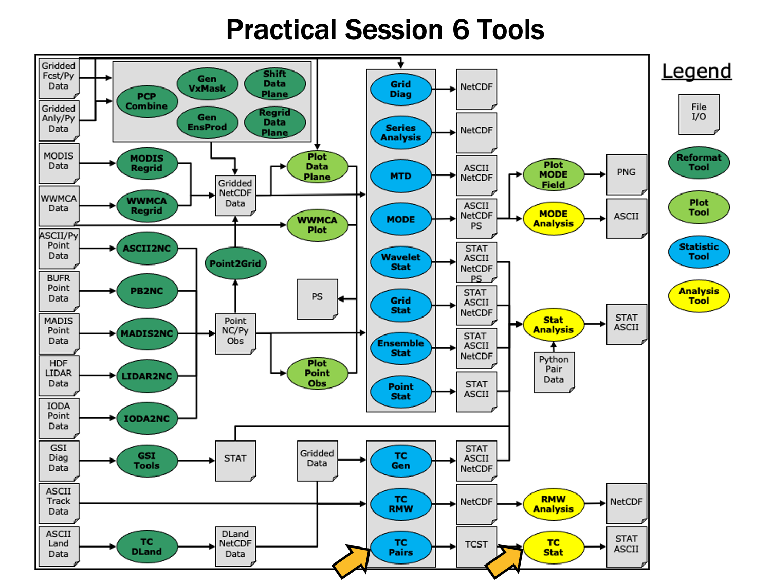
Since you already set up your runtime enviroment in Session 1, you should be ready to go! To be sure, run through the following instructions to check that your environment is set correctly.
Prerequisites: Verify Environment is Set Correctly
Before running the tutorial instructions, you will need to ensure that you have a few environment variables set up correctly. If they are not set correctly, the tutorial instructions will not work properly.
EDIT AFTER COPYING and BEFORE HITTING RETURN!
source METplus-5.0.0_TutorialSetup.sh
echo ${METPLUS_BUILD_BASE}
echo ${MET_BUILD_BASE}
echo ${METPLUS_DATA}
ls ${METPLUS_TUTORIAL_DIR}
ls ${METPLUS_BUILD_BASE}
ls ${MET_BUILD_BASE}
ls ${METPLUS_DATA}
METPLUS_BUILD_BASE is the full path to the METplus installation (/path/to/METplus-X.Y)
MET_BUILD_BASE is the full path to the MET installation (/path/to/met-X.Y)
METPLUS_DATA is the location of the sample test data directory
ls ${METPLUS_BUILD_BASE}/ush/run_metplus.py
See the instructions in Session 1 for more information.
You are now ready to move on to the next section.
MET Tool: TC-Pairs
MET Tool: TC-Pairs
TC-Pairs Tool: General
TC-Pairs Functionality
The TC-Pairs tool provides position and intensity information for tropical cyclone forecasts in Automated Tropical Cyclone Forecast System (ATCF) format. Much like the Point-Stat tool, TC-Pairs produces matched pairs of forecast model output and an observation dataset. In the case of TC-Pairs, both the model output and observational dataset (or reference forecast) must be in ATCF format. TC-Pairs produces matched pairs for position errors, as well as wind, sea level pressure, and distance to land values for each input dataset.
TC-Pairs Usage
View the usage statement for TC-Pairs by simply typing the following:
| Usage: tc_pairs | ||
| -adeck source | Input ATCF format track files | |
| -edeck source | Input ATCF format ensemble probability files | |
| -bdeck source | Input ATCF format observation (or reference forecast) file path/name | |
| -config file | Configuration file | |
| [-out_base] | path of output file base | |
| [-log_file] | name of log associated with tc_pairs output | |
| [-v level] | Level of logging (optional) |
At a minimum, the input ATCF format -adeck (or -edeck) source, the input ATCF format -bdeck source, and the configuration -config file must be passed in on the command line.
The -adeck, -edeck, and -edeck options can be set to either a specific file name or a top-level directory which will be searched for files ending in ".dat".
Input format
Input format
TC-Pairs input data format
As mentioned previously, the input to TC-Pairs is two ATCF format files, in addition to the distance_to_land.nc file generated with the TC-Dland tool. The ATCF file format is a comma-separated ASCII file containing the following fields:
| Basin | basin | |
| CY | annual cyclone number (1-99) | |
| YYYYMMDDHH | Date - Time - Group | |
| TECHNUM/MIN | Objective sorting technique number, minutes in Best Track | |
| TECH | acronym for each objective technique | |
| TAU | forecast period | |
| LatN/S | Latitude for the date time group | |
| LonE/W | Longitude for date time group | |
| VMAX | Maximum sustained wind speed | |
| MSLP | Minimum sea level pressure | |
| TY | Highest level of tropical cyclone development | |
| RAD | wind intensity for the radii at 34, 50, 64 kts | |
| WINDCODE | radius code | |
| RAD1 | full circle radius of wind intensity, 1st quadrant wind intensity | |
| RAD2 | radius of 2nd quadrant wind intensity | |
| RAD3 | radius of 3rd quadrant wind intensity | |
| RAD4 | radius of 4th quadrant wind intensity | |
| ... |
These are the first 17 columns in the ATCF file format. MET-TC requires the input file has all 17 comma-separated columns present (although valid data is not required). For a full list of the columns as well as greater detail on the file format, see: http://www.nrlmry.navy.mil/atcf_web/docs/database/new/abdeck.txt
Model data must be run through a vortex tracking algorithm prior to becoming input for MET-TC. Running a vortex tracker is outside the scope of this tutorial, however a freely available and supported vortex tracking software is available at:https://dtcenter.org/community-code/gfdl-vortex-tracker/download
If users choose to use operational model data for input to MET-TC, all U.S. operational model output in ATCF format can be found at: ftp://ftp.nhc.noaa.gov/atcf/archive. Finally, the most common use of MET-TC is to use the best track analysis (used as observations) to generate pairs between the model forecast and the observations. Best track analyses can be found at the same link as the operational model output.
Open files aal112017.dat (model data) and bal112017.dat (BEST track). Take a look at the columns and gain familiarity with ATCF format. These files are input ATCF files for TC-Pairs.
In addition to the files above, data from five total storms over hurricane seasons 2011-2012 in the AL basin will be used to run TC-Pairs. Rather than running a single storm, these storms were chosen to provide a larger sample size to provide more robust statistics.
- aal092011: Irene
- aal182011: Rina
- aal052012: Ernesto
- aal092012: Isaac
- aal182012: Sandy
Configure
Configure
TC-Pairs Tool: Configure
Start by making an output directory for TC-Pairs and changing directories:
cd ${METPLUS_TUTORIAL_DIR}/output/met_output/tc_pairs
Like the Point-Stat tool, the TC-Pairs tool is controlled by the contents of the configuration file passed to it on the command line. The default TC-Pairs configuration file may be found in the data/config/TCPairsConfig_default file.
The configurable items for TC-Pairs are used to specify which data are ingested and how the input data are filtered. The configurable items include specifications for the following:
- All model names to include in matched pairs
- Storms to include in verification: parsed by storm_id, basin, storm_name, cyclone
- Date/Time/Space restrictions: initialization time, valid time, lead time, masking
- User defined consensus forecasts
- Thresholds over watch/warning status of storm
The first step is to set-up the configuration file. Keep in mind, TC-Pairs should be run with the largest desired sample in mind to minimize re-running this tool! First, make a copy of the default:
Next, open up the TCPairsConfig_tutorial_run file for editing and modify it as follows:
basin = [ "AL" ];
To identify the models that we want to verify, as well as the basin. The three models identified are all U.S. operational models: HWRF, GFS (AVNO), and GFDL. Any field left blank will assume no restrictions.
{
name = "CONS";
members = [ "HWRF", "AVNO", "GFDL" ];
required = [ false, false, false ];
min_req = 2;
}
];
To compute a user defined consensus named "CONS". The membership of the consensus are the three listed models, none are required, but 2 must be present to calculate the consensus.
To only keep pairs that are the intersection of the model forecast and observation.
Next, save the TCPairsConfig_tutorial_run file and exit the text editor.
This run uses the default distance to land output file. Run ncview to see it:
Water points have distance to land values greater than 0 while land points have distances <= 0.
Run
Run
TC-Pairs Tool: Run
Next, run TC-Pairs to compare all three ATCF forecast models specified in configuration file to the ATCF format best track analysis. Run the following command line:
-adeck ${METPLUS_DATA}/met_test/atcf_data/aal*dat \
-bdeck ${METPLUS_DATA}/met_test/atcf_data/bal*dat \
-config TCPairsConfig_tutorial_run \
-out tc_pairs \
-v 2
TC-Pairs is now grabbing the model data we requested in the configuration file, generating the consensus, and performing the additional filtering criteria. It should take approximate 20 seconds to run. You should see several status messages printed to the screen to indicate progress.
There should be an output file "tc_pairs.tcst" in the directory, where .tcst stands for TC statistics. The next page will describe what is in the file.
Output
Output
TC-Pairs Tool: Output
The output of TC-Pairs is an ASCII file containing matched pairs for each of the models requested. In this example, the output is written to the tc_pairs.tcst file as we requested on the command line. This output file is in TCST format, which is similar to the STAT output from the Point-Stat and Grid-Stat tools. For more header information on the TCST format, see the tc_pairs output section of the MET User's Guide.
- In the kwrite editor, select Settings->Configure Editor, de-select Dynamic Word Wrap and click OK.
- In the vi editor, type the command :set nowrap. To set this as the default behavior, run the following command:
Open tc_pairs.tcst
- Notice this is a simple ASCII file with rows for each matched pair for a single valid time and similar to the MPR line type written by other tools.
- Any field that has A in the column name (such as AMAX_WIND, ALAT) indicate the model forecast.
- Any field that has B in the column name (such as BMAX_WIND, BLAT) indicate the observation field (Best Track).
- The TK_ERR, X_ERR, Y_ERR, ALTK_ERR, CRTK_ERR columns are calculated track error, X component position error, Y component postion error, along track error, and cross track error, respectively.
- Columns 34-63 are the 34-, 50-, and 64-kt wind radii for each quadrant.
MET Tool: TC-Stat
MET Tool: TC-Stat
TC-Stat Tool: General
TC-Stat Functionality
The TC-Stat tool reads the .tcst output file(s) of the TC-Pairs tool. This tools provides the ability to further filter the TCST output files as well as summarize the statistical information. The TC-Stat tool reads .tcst files and runs one or more analysis jobs on the data. TC-Stat can be run by specifying a single job on the command line or multiple jobs using a configuration file. The TC-Stat tool is very similar to the Stat-Analysis tool. The two analysis job types are summarized below:
- The filter job simply filters out lines from one or more TCST files that meet the filtering options specified.
- The summary job operates on one column of data from TCST file. It produces summary information for that column of data: mean, standard deviation, min, max, and the 10th, 25th, 50th, 75th, and 90th percentiles, independence time, and frequency of superior performance.
- The rirw job identifies rapid intensification or weakening events in the forecast and analysis tracks and applies categorical verification methods.
- The probrirw job applies probabilistic verification methods to evaluate probability of rapid inensification forecasts found in edeck's.
TC-Stat Usage
View the usage statement for TC-Stat by simply typing the following:
| Usage: tc_stat | ||
| -lookin path | TCST file or top-level directory containing TCST files (where TC-Pairs output resides). It allows the use of wildcards (at least one tcst file is required). | |
| [-out file] | Output path or specific filename to which output should be written rather than the screen (optional). | |
| [-log file] | Outputs log messages to the specified file | |
| [-v level] | Level of logging | |
| [-config config_file] | [JOB COMMAND LINE] (Note: "|" means "or") | ||
| [-config config_file] | TCStat config file containing TC-Stat jobs to be run. | |
| [JOB COMMAND LINE] | Arguments necessary to perform a TC-Stat job. |
At a minimum, you must specify at least one directory or file in which to find TCST data (using the -lookin path command line option) and either a configuration file (using the -config config_file command line option) or a job command on the command line.
Configure
Configure
TC-Stat Tool: Configure
Start by making an output directory for TC-Stat and changing directories:
cd ${METPLUS_TUTORIAL_DIR}/output/met_output/tc_stat
The behavior of TC-Stat is controlled by the contents of the configuration file or the job command passed to it on the command line. The default TC-Stat configuration may be found in the data/config/TCStatConfig_default file. Make a copy of the default configuration file and make following modifications:
Open up the TCStatConfig_tutorial file for editing with your preferred text editor.
bmodel = [ "BEST" ];
event_equal = TRUE;
To only parse over two of the three model names in the tc_pairs.tcst file. The event_equal=TRUE flag will keep pairs for specified forecast valid and lead times that are only in both HWRF and GFDL pairs.
Many of the filter options are left blank, indicating TC-Stat should parse over all available fields. You will notice many more available filter options beyond what was available with the TCPairsConfig.
This will create a job that filters out TCST lines based on the job's criteria (this example has no criteria listed, so all TCST lines will be used) and place them into the file indicated by -dump_row.
Run on TC-Pairs output
Run on TC-Pairs output
TC-Stat: Run on TC-Pairs output
Run the TC-Stat using the following command:
-lookin ../tc_pairs/tc_pairs.tcst \
-config TCStatConfig_tutorial -v 3
Open the output file tc_stat.tcst. We can see that this filter job simply event equalized the two models specified in amodel.
Let's try to filter further, this time using the command line rather than the configuration file:
-job filter -lookin ../tc_pairs/tc_pairs.tcst \
-dump_row tc_stat2.tcst \
-water_only TRUE \
-column_str LEVEL HU,TS,TD,SS,SD \
-event_equal TRUE \
-match_points TRUE -v 3
Here, we ran a filter job at the command line: only keeping tracks over water (not encountering land) and with categories Hurricane (HU), Tropical Storm (TS), Tropical Depression (TD), Subtropical Storm (SS), and Subtropical Depression (SD).
Open the output file tc_stat2.tcst: notice fewer lines have been kept. Look at the "LEVEL" column ... note all the non-tropical and subtropical level classifications have been filtered out of the sample.
Also, find the columns ADLAND and BDLAND. All these values are now positive, meaning the tracks over land (negative values) have been filtered.
With the filtering jobs mastered, lets give the second type of job - summary jobs - a try!
Run on TC-Pairs output
Run on TC-Pairs output
TC-Stat: Run on TC-Pairs output
Now, we will run a summary job using TC-Stat on the command line using the following command:
-job summary -lookin ../tc_pairs/tc_pairs.tcst \
-amodel HWRF,GFDL \
-by LEAD,AMODEL \
-column TK_ERR \
-event_equal TRUE \
-out tc_stat_summary.tcst
Open up the file tc_stat_summary.tcst. Notice this output is much different from the filter jobs.
The track data is event equalized for the HWRF and GFDL models, and summary statistics are produced for the TK_ERR column for each model by lead time.
Plotting with R
Plotting with R
TC-Stat: Plotting with R
In this section, you will use the R statistics software package to produce a plot of a few results. R was introduced in practical session 1.
The MET release includes a number of plotting tools for TC graphics. All of the Rscripts are included with the MET distribution in the Rscripts directory. The script for TC graphics is plot_tcmpr.R, which uses the TCST output files from TC-Pairs as input. At this time, there are two additional environment variables that need to be set to make this work. They are MET_INSTALL_DIR and MET_BASE. To get the usage statement, type:
For Bash:
export MET_BASE=${MET_INSTALL_DIR}/share/met
Rscript ${MET_BASE}/Rscripts/plot_tcmpr.R
For C-shell:
setenv MET_BASE ${MET_INSTALL_DIR}/share/met
Rscript ${MET_BASE}/Rscripts/plot_tcmpr.R
The TC-Stat tool can be called from the Rscript to do additional filter jobs on the TCST output from TC-Pairs. This can be done on the command line by calling a filter job (following tc-stat), or a configuraton file can be used to select filtering criteria. A default configuration file can be found in Rscripts/include/plot_tcmpr_config_default.R.
The configuration file also includes various plot types to generate: MEAN, MEDIAN, SCATTER, REFPERF, BOXPLOT, and RANK. All of the plot commands can be called on the command line as well as with the configuration file. Plots are configurable (title, colors, axis labels, etc) either by modifying the configuration file or setting options on the command line. To run from the command line:
-lookin ../tc_pairs/tc_pairs.tcst \
-filter "-amodel HWRF,CONS" \
-dep "TK_ERR" \
-series AMODEL HWRF,CONS \
-plot MEAN,BOXPLOT,RANK \
-outdir .
This plots the track error for two models: HWRF and CONS. CONS is the user defined consensus you generated in TC-Pairs.
Next, open up the output *png files:
display TK_ERR_mean.png &
display TK_ERR_rank.png &
The script produces the three plot types called in the configuration file:
- Boxplot showing distribution of errors for a homogeneous sample of the two models (TK_ERR_boxplot.png).
- Mean Errors with 95% CI for the same sample (TK_ERR_mean.png).
- Rank plot indicating performance of HWRF model relative to CONS (TK_ERR_rank.png).
METplus Use Case: TC-Pairs
METplus Use Case: TC-Pairs
The TCPairs use case utilizes the MET TC-Pairs tool.
Optional: Refer to the MET Users Guide for a description of the MET tools used in this use case.
Optional: Refer to the METplus Config Glossary section of the METplus Users Guide for a reference to METplus variables used in this use case.
There is an example of using TC-Pairs to match Extratropical Cyclones as well as Tropical Cyclones
TCPairs_tropical.conf
MODEL = MYNN, H19C, H19M, CTRL, MYGF
TC_PAIRS_CYCLONE = 06
TC_PAIRS_ADECK_INPUT_DIR = {INPUT_BASE}/met_test/new/hwrf/adeck
TC_PAIRS_OUTPUT_DIR = {OUTPUT_BASE}/tc_pairs
TC_PAIRS_ADECK_TEMPLATE = {model?fmt=%s}/*{cyclone?fmt=%s}l.{date?fmt=%Y%m%d%H}.trak.hwrf.atcfunix
Let's take a look at the data to understand why the configuration file is set up the way it is. If you recall, the {INPUT_BASE} is set in tutorial.conf as ${METPLUS_DATA}, so we will look there:
The output from this command will return four separate directories, each with their own collection of track files. Those four directories are:
H19C
H19M
MYNN
An example of the track files found in each of these directories is:
${METPLUS_BUILD_BASE}/parm/use_cases/met_tool_wrapper/TCPairs/TCPairs_tropical.conf \
${METPLUS_TUTORIAL_DIR}/tutorial.conf \
config.OUTPUT_BASE=${METPLUS_TUTORIAL_DIR}/output/TCPairs
Let's look at the output file:
vi ${METPLUS_TUTORIAL_DIR}/output/TCPairs/tc_pairs/tc_pairs_al2018083012.dat.tcst
vi ${METPLUS_TUTORIAL_DIR}/output/TCPairs/tc_pairs/tc_pairs_al2018083018.dat.tcst
You will notice that there are two models configurations included in the first file for Hurricane Florence, CTRL and MYNN and the line type written out is TCMPR indicate it is the matched pair information. If you open up the third file, you'll notice that there is only the CTRL model listed.
less ${METPLUS_DATA}/met_test/new/hwrf/adeck/H19C/six06l.2018083018.trak.hwrf.atcfunix
less ${METPLUS_DATA}/met_test/new/hwrf/adeck/H19M/six06l.2018083012.trak.hwrf.atcfunix
less ${METPLUS_DATA}/met_test/new/hwrf/adeck/MYNN/six06l.2018083018.trak.hwrf.atcfunix
You will see that in the files are in the ATCF file format. Also note: in the files in the CTRL directory, the model listed in the 5th column is HLAT. Similarly, in the H19C directory, the model is CTRL; in the H19M directory it is MYNN, and in the MYNN directory, it is HLMY. While this is confusing in some ways, it does demonstrate that the TC-Pairs tool does not look at the directory structure and naming convention of the input files, but rather the model information included in the ATCF "a-decks", which is traditional naming convention for files with forecast tracks.
${METPLUS_TUTORIAL_DIR}/user_config/TCPairs_run2.conf
The TC_PAIRS_ADECK_TEMPLATE includes MODEL in the path, so we will leave MYNN and CTRL in the list.
${METPLUS_TUTORIAL_DIR}/user_config/TCPairs_run2.conf \
${METPLUS_TUTORIAL_DIR}/tutorial.conf \
config.OUTPUT_BASE=${METPLUS_TUTORIAL_DIR}/output/TCPairs_run2
Review output
vi ${METPLUS_TUTORIAL_DIR}/output/TCPairs_run2/tc_pairs/tc_pairs_al2018083012.dat.tcst
vi ${METPLUS_TUTORIAL_DIR}/output/TCPairs_run2/tc_pairs/tc_pairs_al2018083018.dat.tcst
You will notice that now all models are included in the appropriate files. Also note that all of the forecasts leads from 000000 to 1260000 are included in the 10th column.
METplus Use Case: TC-Stat
METplus Use Case: TC-Stat
The TCPairs use case utilizes the MET TC-Pairs tool.
Optional: Refer to the MET Users Guide for a description of the MET tools used in this use case.
Optional: Refer to the METplus Config Glossary section of the METplus Users Guide for a reference to METplus variables used in this use case.
Change to the ${METPLUS_TUTORIAL_DIR}
- See what TCPairs use cases are available in met_tool_wrapper directory and run one
There is an example of using TC-Stat with no delineation between Extratropical Cyclones as well as Tropical Cyclones
TC_STAT_JOB_ARGS = -job summary -line_type TCMPR -column 'ASPEED' -dump_row {TC_STAT_OUTPUT_DIR}/tc_stat_summary.tcst
TC_STAT_INIT_BEG = 20150301
TC_STAT_INIT_END = 20150304
TC_STAT_LANDFALL_BEG = -24
TC_STAT_LANDFALL_END = 00
TC_STAT_LOOKIN_DIR = {INPUT_BASE}/met_test/tc_pairs
This use case is focused on summarizing the ASPEED data including data from 24 hours before landfall. Keep in mind the summary information will be written out. Also, because the -dump_row flag was set, output will be placed in the file {TC_STAT_OUTPUT_DIR}/tc_stat_summary.tcst
- Run the use case:
${METPLUS_BUILD_BASE}/parm/use_cases/met_tool_wrapper/TCStat/TCStat.conf \
${METPLUS_TUTORIAL_DIR}/tutorial.conf \
config.OUTPUT_BASE=${METPLUS_TUTORIAL_DIR}/output/TCStat
-
Review the output and input files:
Look at the output written to the directory specified as TC_STAT_OUT_DIR
You will notice this looks very similar to output from TCPairs, confirmed by noting the LINE_TYPE is TCMPR. While this is helpful, the outcome of the SUMMARY job is part of standard output from the tool, unless the -out flag is used when calling the tool. Standard output will be found in the location specified by the TC_STAT_OUTPUT_TEMPLATE. For this example, the file will be named job.out
Open the standard output file in ${METPLUS_TUTORIAL_DIR}/output/TCStat/, with the filename job.out. Inside, you'll find:
SUMMARY: 'ASPEED' 351 0 NA NA NA NA NA NA NA NA NA NA NA NA NA NA NA NA 0 0 0 NA
The headers indicate that this information includes details about the distribution of data as well as measures to generate plots of Frequency of Superior Performance. The description of each column can be found at: https://met.readthedocs.io/en/latest/Users_Guide/index.html. The other notable result is that most columns are listed as NA. This is because the -column setting is listed as 'ASPEED' with quotes around the column name. The quotes appears to be an error, probably a remnant of a previous METplus version. Let's change that and see what happens.
- Copy METplus config file, modify and re-run
${METPLUS_TUTORIAL_DIR}/user_config/TCStat_run2.conf
${METPLUS_TUTORIAL_DIR}/user_config/TCStat_run2.conf \
${METPLUS_TUTORIAL_DIR}/tutorial.conf \
config.OUTPUT_BASE=${METPLUS_TUTORIAL_DIR}/output/TCStat_run2
- Review output
SUMMARY: ASPEED 351 351 -12.04558 -44.41459 20.32342 309.41037 -860 -384 -242 -95 226 377 886 468 1746 -4228 NA NA 0 0 0 NA
SUMMARY: TK_ERR 351 351 42.82123 37.93854 47.70392 46.67289 0 0 11.16231 27.10901 61.31199 97.229 370.00025 50.14968 370.00025 15030.25036 NA NA 0 0 0 NA
The values of ASPEED and TK_ERR are now available. Let's take one more step to demonstrate additional capability.
- Copy METplus config file, modify and re-run
${METPLUS_TUTORIAL_DIR}/user_config/TCStat_run3.conf
${METPLUS_TUTORIAL_DIR}/user_config/TCStat_run3.conf \
${METPLUS_TUTORIAL_DIR}/tutorial.conf \
config.OUTPUT_BASE=${METPLUS_TUTORIAL_DIR}/output/TCStat_run3
- Review output
Open standard output file in ${METPLUS_TUTORIAL_DIR}/output/TCStat_run3 under the name job.out and scroll down to the bottom.
SUMMARY: AMAX_WIND -109 8 8 26.75 24.66593 28.83407 2.49285 23 24.4 25.75 26 28.25 29.6 31 2.5 8 214 060000 054200 0 0 0 NA
SUMMARY: AMAX_WIND -118 3 3 36.33333 24.07937 48.58729 4.93288 33 33.2 33.5 34 38 40.4 42 4.5 9 109 060000 070000 0 0 0 NA
SUMMARY: AMAX_WIND -119 24 24 35.125 32.55402 37.69598 6.08857 24 25.6 30.75 36.5 39.25 42 45 8.5 21 843 NA NA 0 0 0 NA
...
SUMMARY: AMAX_WIND 79 15 15 18.13333 16.37131 19.89535 3.18179 14 15 15.5 17 20 22.8 24 4.5 10 272 NA NA 0 0 0 NA
SUMMARY: AMAX_WIND 83 8 8 20.5 18.82796 22.17204 2 19 19 19 19.5 21.5 23.3 24 2.5 5 164 060000 070730 0 0 0 NA
...
SUMMARY: TK_ERR 51 9 9 19.98849 6.43677 33.54021 17.63013 0 2.5649 6.71828 18.23421 21.86675 47.58604 49.27937 15.14847 49.27937 179.89644 060000 100000 0 0 0 NA
SUMMARY: TK_ERR 54 32 32 29.61144 19.00544 40.21744 30.61107 0 0.31881 8.17406 19.52752 42.21794 80.32842 111.04562 34.04387 111.04562 947.56606 NA NA 0 0 0 NA
There are now 48 lines with lines summarizing AMAX_WIND and TK_ERR across 24 STORM_NAMEs. The information for FSP columns is zero because there is only data for 1 model being summarized.
METplus Use Case: Track and Intensity Plotting
METplus Use Case: Track and Intensity Plotting
METplus Use Case: Track and Intensity TCMPR (Tropical Cyclone Matched Pair) Plotter
This is a wrapper to the MET plot_tcmpr.R, based on R-project Statistical package Rscript. This Rscript will be deprecated in a future METplus release.
Review: Take a look at the following settings.
The default image resolution for the plot_tcmpr.R Rscript is set to 300, for print quality, but quite large for display purposes. The following is an R config file that is passed to the Rscript and changes the default and reduces the image size. It is a simple one line file, but go and take a look.
The plot_tcmpr.R script knows to read this TCMPRPlotterConfig_Customize R config file since it is defined in the TCMPRPlotter.conf file.
Note: If you modify the TCMPR_PLOTTER_CONFIG_FILE variable and leave it undefined (not set), then no configuration file will be read by the R script and the default setting of img_res=300 will be used.
TCMPR_DATA - the path to the input data, in this example, we are using the data in the TC_PAIRS_DIR directory.
MODEL_DATA_DIR - path to the METplus input data.
TRACK_DATA_DIR - path to the METplus input data.
Optional, Refer to the TC-Stat tool example section of the MET Users Guide for a description of plot_tcmpr.R
If you wish, refer to the Format Information for TCMPR output line type table, for a tabular description of the TC-Pairs output TCST format. After running this Track and Intensity example, you can view the TC-Pairs TCST output files generate by this example under your ${METPLUS_TUTORIAL_DIR}/output/track_and_intensity/tc_pairs directory while comparing to the information in the table.
The tcmpr defaults are used for any conf settings left as, unset, For example as: XLAB =
The current settings in the conf files are ok and no changes are required. However, after running the exercise feel free to experiment with these settings.
The R script that Track and Intensity runs is located in the MET installation; share/met/Rscripts/plot_tcmpr.R. The usage statement with a short description of the options for plot_tcmpr.R can be obtained by typing:
with no additional arguments. The usage statement can be helpful when setting some of the option in METplus, below is a description of these settings.
- CONFIG_FILE is a plotting configuration file
- PREFIX is the output file name prefix.
- TITLE overrides the default plot title. Bug: CAN_NOT_HAVE_SPACES
- SUBTITLE overrides the default plot subtitle.
- XLAB overrides the default plot x-axis label.
- YLAB overrides the default plot y-axis label.
- XLIM is the min,max bounds for plotting the X-axis.
- YLIM is the min,max bounds for plotting the Y-axis.
- FILTER is a list of filtering options for the tc_stat tool.
- FILTERED_TCST_DATA_FILE is a tcst data file to be used instead of running the tc_stat tool.
- DEP_VARS is a comma-separated list of dependent variable columns to plot.
- SCATTER_X is a comma-separated list of x-axis variable columns to plot.
- SCATTER_Y is a comma-separated list of y-axis variable columns to plot.
- SKILL_REF is the identifier for the skill score reference.
- LEGEND is a comma-separted list of strings to be used in the legend.
- LEAD is a comma-separted list of lead times (h) to be plotted.
- RP_DIFF is a comma-separated list of thresholds to specify meaningful differences for the relative performance plot.
- DEMO_YR is the demo year
- HFIP_BASELINE is a string indicating whether to add the HFIP baseline and which version (no, 0, 5, 10 year goal)
- FOOTNOTE_FLAG to disable footnote (date).
- PLOT_CONFIG_OPTS to read model-specific plotting options from a configuration file.
- SAVE_DATA to save the filtered track data to a file instead of deleting it.
- PLOT_TYPES is a comma-separated list of plot types to create:
- BOXPLOT, POINT, MEAN, MEDIAN, RELPERF, RANK, SKILL_MN, SKILL_MD
- for this example, set to MEAN,MEDIAN to generate MEAN and MEDIAN plots.
- SERIES is the column whose unique values define the series on the plot, optionally followed by a comma-separated list of values, including:
ALL, OTHER, and colon-separated groups. - SERIES_CI is a list of true/false for confidence intervals. Optionally followed by a comma-separated list of values, including:
ALL, OTHER, and colon-separated groups.
Run METplus: Run Track and Intensity use case.
Examples: Run the track and intensity plotting script
Generates plots using the MET plot_tcmpr.R Rscript.
Example 1:
In this case, the TCMPRPlotter.conf file is configured to generate MEAN and MEDIAN plot types with TCMPR_PLOTTER_PLOT_TYPES.
Run the following command:
${METPLUS_BUILD_BASE}/parm/use_cases/met_tool_wrapper/TCMPRPlotter/TCMPRPlotter.conf \
${METPLUS_TUTORIAL_DIR}/tutorial.conf \
config.OUTPUT_BASE=${METPLUS_TUTORIAL_DIR}/output/track_and_intensity
The following directory lists the files generated from running these use cases:
AMAX_WIND-BMAX_WIND_boxplot.png
AMAX_WIND-BMAX_WIND_mean.png
AMAX_WIND-BMAX_WIND_median.png
AMSLP-BMSLP_mean.png
AMSLP-BMSLP_median.png
TK_ERR_mean.png
TK_ERR_median.png
Example 2:
Copy the TCMPRPlotter.conf file to the user_config directory:
${METPLUS_TUTORIAL_DIR}/user_config/TCMPRPlotter_boxplot.conf
Open the new conf file with an editor and change the list of plot types to only include BOXPLOT.
Change this line (around line 65):
to
Close the file and rerun METplus:
${METPLUS_TUTORIAL_DIR}/user_config/TCMPRPlotter_boxplot.conf \
${METPLUS_TUTORIAL_DIR}/tutorial.conf \
config.OUTPUT_BASE=${METPLUS_TUTORIAL_DIR}/output/track_and_intensity_boxplot
The following directory lists the additional files generated from running this use case:
AMAX_WIND-BMAX_WIND_boxplot.png
AMSLP-BMSLP_boxplot.log
AMSLP-BMSLP_boxplot.png
TK_ERR_boxplot.log
TK_ERR_boxplot.png
To view the png images generated by running these examples, use the display command.
cd to your OUTPUT_BASE/tcmpr_plots directory.
display AMAX_WIND-BMAX_WIND_mean.png &
display AMAX_WIND-BMAX_WIND_median.png &
display AMAX_WIND-BMAX_WIND_boxplot.png> &
End of Session 6
End of Session 6
End of Session 6
Congratulations! You have completed Session 6!
Session 7: Feature Relative Use Cases
Session 7: Feature Relative Use Cases
METplus Practical Session 7
This session will cover two METplus feature relative use cases.
Prerequisites: Verify Environment is Set Correctly
Before running the tutorial instructions, you will need to ensure that you have a few environment variables set up correctly. If they are not set correctly, the tutorial instructions will not work properly.
EDIT AFTER COPYING and BEFORE HITTING RETURN!
source METplus-5.0.0_TutorialSetup.sh
echo ${METPLUS_BUILD_BASE}
echo ${MET_BUILD_BASE}
echo ${METPLUS_DATA}
ls ${METPLUS_TUTORIAL_DIR}
ls ${METPLUS_BUILD_BASE}
ls ${MET_BUILD_BASE}
ls ${METPLUS_DATA}
METPLUS_BUILD_BASE is the full path to the METplus installation (/path/to/METplus-X.Y)
MET_BUILD_BASE is the full path to the MET installation (/path/to/met-X.Y)
METPLUS_DATA is the location of the sample test data directory
ls ${METPLUS_BUILD_BASE}/ush/run_metplus.py
If more information is needed see the instructions in Session 1 for more information.
You are now ready to move on to the next section.
Click on a use case below to get started.
METplus Use Case: Feature Relative (Series-Analysis by Initialization Time)
METplus Use Case: Feature Relative (Series-Analysis by Initialization Time)
METplus Use Case: Feature Relative (Series-Analysis by init)
Setup
In this exercise, you will perform a series analysis based on the init time of your sample data. This use case focuses on using the latitude and longitude pairs for a "feature", such as a tropical cyclone or extra-tropical cyclone, to identify a user-specified tile around the feature. The tiles are then used to compute statistics using Series_Analysis. Therefore, this use-case utilizes the MET Tc-Pairs, Tc-Stat, and Series-Analysis tools, and the METplus wrappers: TcPairs, ExtractTiles, TcStat, and SeriesAnalysis. Please refer to the MET Users Guide for a description of the MET tools and the METplus Users Guide for more details about the wrappers.
Review Use Case Configuration File: feature_relative.conf
View the file and study the configuration variables that are defined.
Note the configuration settings for this complex use-case. The PROCESS_LIST contains 5 items, 2 of which are the same wrapper, TCStat. Since METplus version 4.0.0 was released, users have had the ability to run multiple instances of a given tool using an instance name. The METplus User's Guide describes in detail how to use Instance Names in the Process List to configure two or more instances of the same tool with different settings.
For this example, the [for_series_analysis] instance of TCStat, which runs after the initial TCStat instance and an ExtractTiles instance, will inherit all of the settings from the initial TCStat instance. Then, it will override those settings with any of the settings found in the [for_series_analysis] section. Looking at the configuration file, we see the following:
TC_STAT_OUTPUT_DIR = {SERIES_ANALYSIS_OUTPUT_DIR}
TC_STAT_LOOKIN_DIR = {EXTRACT_TILES_OUTPUT_DIR}
This indicates that the TC_STAT_JOB_ARGS, TC_STAT_OUTPUT_DIR, and TC_STAT_LOOKIN_DIR will be overridden with the provided values.
The SERIES_ANALYSIS_STAT_LIST is set to four statistics, but can be set to many more. The size of the tiles are configurable using the EXTRACT_TILES settings. Also, note that variables in feature_relative.conf reference other variables you defined in other configuration files. For example:
This references OUTPUT_BASE which you set in the METplus defaults configuration file (${METPLUS_BUILD_BASE}/parm/metplus_config/defaults.conf). METplus config variables can reference other config variables, even if they are defined in a config file that is read afterwards.
Run METplus
Change to the METplus Tutorial Directory:
Run the following command. Use config.OUTPUT_BASE to change the output directory from the command line:
${METPLUS_BUILD_BASE}/parm/use_cases/model_applications/medium_range/TCStat_SeriesAnalysis_fcstGFS_obsGFS_FeatureRelative_SeriesByInit.conf \
${METPLUS_TUTORIAL_DIR}/tutorial.conf \
config.OUTPUT_BASE=${METPLUS_TUTORIAL_DIR}/output/feature_relative_by_init
You will see output streaming to your screen. This may take up to 4 minutes to complete. METplus is finished running when control returns to your terminal console and you see the following text:
Review the Output Files
You should have output files in the following directories from the intermediate wrappers TcPairs, ExtractTiles, and TcStat, respectively:
extract_tiles
track_data_atcf
and the output of interest, from the SeriesAnalysis wrapper:
which has a directory corresponding to the date(s) of data in the data window. This area also includes the logs and a tmp directory:
and under that directory are subdirectories named by the storm. They begin with ML. Below are a few examples:
ML1201042014, etc.
and under each of those directories lies the files of interest:
series_analysis_files_obs_ML1201042014_init_20141214000000_valid_ALL_lead_ALL.txt
series_TMP_Z2_FBAR.png
series_TMP_Z2_FBAR.ps
series_TMP_Z2_ME.png
series_TMP_Z2_ME.ps
series_TMP_Z2.nc
series_TMP_Z2_OBAR.png
series_TMP_Z2_OBAR.ps
series_TMP_Z2_TOTAL.png
series_TMP_Z2_TOTAL.ps
The series_analysis_files_obs_ML########## (where ########## is the storm) is a text file that contains a list of the observation data included in the series analysis.
The series_analysis_files_fcst_ML########## (where ########## is the storm) is a text file that contains a list of forecast data included in the series analysis.
The .nc files are the series analysis output generated from the MET series_analysis tool.
The .png and .ps files are graphics files that can be viewed using display or ghostview, respectively:
or
Note: the & is used to run this command in the background
Review the Log File
A log file is generated in your logging directory: ${METPLUS_TUTORIAL_DIR}/output/feature_relative_by_init/logs. The filename contains the timestamp corresponding to the current day. To view the log file:
Review the Final Configuration File
The final configuration file is metplus_final.conf. This contains all of the configuration variables used in the run.
METplus Use Case: Feature Relative (Series-Analysis by Lead Time with Forecast Hour Grouping)
METplus Use Case: Feature Relative (Series-Analysis by Lead Time with Forecast Hour Grouping)
METplus Use Case: Feature Relative (Series-Analysis by lead, by forecast hour grouping)
Setup
In this exercise, you will perform a series analysis based on the lead time (forecast hour) of your sample data and organize your results by forecast hour groupings. This use case utilizes the MET Tc-Pairs, Tc-Stat, and Series-Analysis tools, and the METplus wrappers: TcPairs, ExtractTiles, TcStat, and SeriesAnalysis. Please refer to the MET User's Guide for a description of the MET tools and the METplus Users Guide for more details about the wrappers. Please note that the METplus User's Guide is a work-in-progress and may have missing content.
Change to the METplus Tutorial Directory:
Review Use Case Configuration File: series_by_lead_by_fhr_grouping.conf
View the file and study the configuration variables that are defined.
Note that the Lead time groupings are specified by the LEAD_SEQ config options.
# forecast lead sequence 1 list (0, 6, 12, 18)
LEAD_SEQ_1 = begin_end_incr(0,18,6)
LEAD_SEQ_1_LABEL = Day1
# forecast lead sequence 2 list (24, 30, 36, 42)
LEAD_SEQ_2 = begin_end_incr(24,42,6)
LEAD_SEQ_2_LABEL = Day2
This references OUTPUT_BASE which you set in the METplus default configuration file (metplus_config/defaults.conf). METplus config variables can reference other config variables, even if they are defined in a config file that is read afterwards.
Run METplus
Run the following command:
${METPLUS_TUTORIAL_DIR}/tutorial.conf \
${METPLUS_BUILD_BASE}/parm/use_cases/model_applications/medium_range/TCStat_SeriesAnalysis_fcstGFS_obsGFS_FeatureRelative_SeriesByLead.conf \
dir.OUTPUT_BASE=${METPLUS_TUTORIAL_DIR}/output/feature_relative_by_lead_fhr_groupings
You will see output streaming to your screen. This may take up to 3 minutes to complete. When it is complete, your prompt returns.
Review the Output Files
You should have output directories including the following that result from running the wrappers TcPairs, ExtractTiles, and TcStat, respectively:
extract_tiles
tc_pairs
and the output directory of interest, from the SeriesByLead wrapper:
That directory contains the following directories:
Day2
series_animate
Day1 contain the following files:
series_analysis_files_obs_init_ALL_valid_ALL_lead_ALL.txt
series_F000_to_F018_TMP_Z2_FBAR.png
series_F000_to_F018_TMP_Z2_FBAR.ps
series_F000_to_F018_TMP_Z2_ME.png
series_F000_to_F018_TMP_Z2_ME.ps
series_F000_to_F018_TMP_Z2.nc
series_F000_to_F018_TMP_Z2_OBAR.png
series_F000_to_F018_TMP_Z2_OBAR.ps
series_F000_to_F018_TMP_Z2_TOTAL.png
series_F000_to_F018_TMP_Z2_TOTAL.ps
The series_analysis_files_obs_init_ALL_valid_ALL_lead_ALL.txt is a text file that contains a list of the data that is included in the series analysis.
Day2 contains equivalent files for forecast leads 24 to 42.
The .nc files are the series analysis output generated from the MET Series-Analysis tool.
The .png and .ps files are graphics files that can be viewed using display:
or
Note: the & is used to run this command in the background
The series_animate directory contains the gif images of the animations:
series_animate_TMP_Z2_ME.gif
series_animate_TMP_Z2_OBAR.gif
series_animate_TMP_Z2_TOTAL.gif
To watch the animations, go to ${METPLUS_TUTORIAL_DIR}/output/feature_relative_by_lead_fhr_groupings/series_analysis_lead/series_animate, enter the following (if firefox doesn't work you can use animate instead):
Review the Log File
A log file is generated in your logging directory: ${METPLUS_TUTORIAL_DIR}/output/feature_relative_by_lead_fhr_groupings/logs. The filename contains the timestamp corresponding to the current day. To view the log file:
Review the Final Configuration File
The final configuration file is metplus_final.confYYYYMMDDHHMMSS. (where YYYYMMDDHHMMSS refers to year, month, day, hour, minute, second that the file was created.)This contains all of the configuration variables used in the run.
End of Session 7
End of Session 7
End of Session 7
Congratulations! You have completed Session 7!
Session 8: METplus Analysis Tools
Session 8: METplus Analysis Tools
METplus Practical Session 8
This session will cover METplus analysis tools. Click on an item below to get started.
METviewer
METviewer
METviewer: General
METviewer Overview
METviewer is a database and display system for storing and plotting data from the MET .stat and MODE _obj.txt files. It is used heavily within the DTC and by NOAA-GSD and NOAA-EMC. While its distribution is limited, it is available to the community through a Docker container. For more information, please see:
- Numerical Weather Prediction (NWP) Containers DTC tutorial to run WPS, GSI, WRF, UPP, MET, and METviewer with containers.
- METviewer Source Code GitHub repository (https://github.com/dtcenter/metviewer)
- METviewer Container GitHub repository (https://github.com/dtcenter/container-dtc-metviewer)
Here, we will use the publicly available version of METviewer running at NCAR to demonstrate the METviewer webapp.
METviewer reads MET verification statistics from a database and creates plots using the R statistical package. The tool includes a web application that can be accessed from a web browser to create a single plot. The specification for each plot is built using a series of controls and then serialized into XML. For each plot, METviewer generates a SQL query, an R script to create the plot, a flat file containing the data that will be plotted and the plot itself.
METviewer Web Application
The following example can be run using the METviewer instance located at the link below. It is recommended to move the new tab into a new browser window, so that you can view both the example instructions and the METviewer web application side-by-side.
The following pages have instructions for generating two different types of plots:
- A threshold series plot of Accuracy (ACC) and Critical Success Index (CSI)
- A forecast lead time box plot series of MODE object area distributions
Please be sure to follow these instructions in order.
Time Series of Categorical Statistics Plot
Time Series of Categorical Statistics Plot
METviewer: Time Series of Categorical Statistics Plot
The following list shows the setting name and the setting value for each of the controls on the web application. Please go through them in order, starting at the top, setting and checking the controls as suggested. The settings that you need to change are marked in blue. The settings are grouped according to the areas on the web app. If you need more information about the controls, please click the little i in a circle to the right of METviewer X.Y at the very top of the page. This will take you to the METviewer documentation.
- Database: Click on the box named Select databases and from the Verification group, select mv_met_tutorial to make a plot with sample tutorial data.
- Tab: Series - Create a time-series (as we will do here) or threshold-series line plot. The different tabs correspond to the types of plots that METviewer can generate, such as box plots, bar plots, histograms, and ensemble plots.
- Plot Data: Stat - Plot traditional statistics as opposed to MODE object attributes.
- Y1 Axis variables - These controls specify the statistics and curves for the Y1 axis of the plot.
- Y1 Dependent (Forecast) Variables - pairs of forecast variables and statistics to be plotted
- Click the dropdown list and select: APCP_03 to select 3-hourly Accumulated Precipitation
- Click Select attribute stat dropdown list and select: ACC and CSI to plot Accuracy and Critical Success Index
- Y1 Series Variables - specifies the lines on the plot for each dependent variable
- Click the dropdown list and select: MODEL
- Click the Select value dropdown list and select: QPF to output the one model present
- Next, click the + Series Variable button, click the dropdown list, and select: FCST_THRESH
- Click the Select value dropdown list and select: >0.0, >2.54, and >6.35 to plot statistics for 3 categorical thresholds
- Y1 Dependent (Forecast) Variables - pairs of forecast variables and statistics to be plotted
- Y2 Axis Tab - these controls specify the statistics and curves for the Y2 axis of the plot; it is not used in this demonstration
- Fixed Values - field/value pairs that are held constant for all data on the plot
- Click the + Fixed Value button - to add a fixed value selection option
- Click the dropdown list and select VX_MASK
- Click the Select value dropdown list and select: FULL to plot data for FULL model domain (the only one present in this dataset)
- Independent Variable - the x-axis field and values over which the data are displayed on the plot
- Click the dropdown list and select FCST_LEAD
- Click the Select value dropdown list and click the Check all option to select all items
- Statistics
- The Summary radio button tells MET to plot the mean or median of the statistics pulled directly from the database.
- The Aggregation statistics radio button tells METviewer to aggregate contingency table counts or partial sums and compute aggregate summary statistics and confidence intervals.
- Use the default Summary radio button selection
- Series Formatting - settings to control colors, line types, plotting symbols, and confidence intervals
- There should be settings for 6 lines: 3 lines for ACC followed by 3 lines for CSI
- In the Line Color column:
- Set the 1st and 4th lines to the same RED color
- Set the 2nd and 5th lines to the same GREEN color
- Set the 3rd and 6th lines to the same BLUE color
- In the Line Type column:
- Set the 4th, 5th, and 6th lines to dashed
- Plot Formatting - settings that control the appearance of the plot, along with several miscellaneous features
- On the Titles & Labels tab
- set Plot Title to ACC / CSI vs. Lead Time
- set X label to Forecast Lead
- set Y1 label to ACC / CSI
- On the Common tab, select Display Number of Stats
- On the Titles & Labels tab
- Click the Generate Plot button at the top of the page to submit your plot request to the METviewer plotting engine.
Time Series of Categorical Statistics Plot Output
Time Series of Categorical Statistics Plot Output
METviewer: Time Series of Categorical Statistics Plot Output
If you successfully followed the instructions on the previous page, you should see a plot appear in the in the plot tab of the METviewer window. Your plot should look like this PNG IMAGE. And here is the corresponding plot XML File.
Studying the plot shows that the Critical Success Index (CSI) decreases for higher thresholds, as if often the case. This suggests that the forecast models have more skill at lower precipitation thresholds. This contrasts with the story told by the accuracy statistic, which increases as the threshold increases. This can be explained by the simplicity of the accuracy statistic, and the effect that always predicting no event can have for extreme events.
The following section discusses the output that METviewer generates for each plot. Click through the tabs above the METviewer plot to examine each:
- XML Tab: When the Generate Plot button is clicked, the web application serializes the information in the web page controls into an XML document and sends it across the internet to METviewer. This XML document can be used to generate a plot directly from METviewer using the command line interface, also called the batch engine. The batch engine can create many plots from a single XML document, using only small changes. Thus, a good way to use the METviewer web application is to "design" plots and then take the XML for the plot and extend it to create many different plots.
- Log Tab: The METviewer plot engine generates status output as it runs, and this information can be useful for finding problems.
- R script Tab: METviewer uses the R statistics package to generate plots by constructing an R script and running it in R. The R script that is constructed can be saved and modified if the users would like to make changes to the plot that are not supported in METviewer.
- R data Tab: Along with the R script generated by METviewer for the plot, the plot data is stored in a file that is read when the plot is generated in R. This file can be useful for problem solving, since it shows all of the data used in the plot and can be loaded directly into R for analysis.
- SQL Tab: All of the MET verification statistics output is stored in a database, which METviewer searches when it generates a plot. The SQL generated by METviewer to gather the data for a plot can be viewed, in case the user wants to explore or debug using the SQL directly.
Object Based Attribute Area Box Plot
Object Based Attribute Area Box Plot
METviewer: Object Based Attribute Area Box Plot
For the next plot, you'll try out the XML upload feature. Each plot created by METviewer corresponds to an XML file that defines the plot. In this example, you'll load the XML from a previous plot and regenerate it.
- Right click on this XML file, select the Save Link As option, and save the file to your machine.
- In the METviewer window, click on the Load XML button in the top-right corner.
- In the Upload plot XML file dialog box, click the Browse button, and navigate the location of the XML file.
- Select the XML file, click the Open button, and then the OK button.
- METviewer will now populate all of the selections with those specified in that XML file.
- Lastly, click the Generate Plot button at the top of the page to create the image. Your plot should look like this PNG Image.
This plot shows the area of MODE objects defined for 1-hourly accumulated precipitation thresholded at 0.1 inch. The data has been filtered down to the 00Z initialization and the areas are plotted by lead time. Each lead time has 3 boxplots: core1 in red, core2 in blue, and the observations in gray. The numbers in black across the top show the number of objects plotted for each lead time.
Note that we have only plotted the observations once since they should be the same for both models. Look in the Series Formatting section at the bottom of the METviewer webapp in the Hide column to see that we're hiding the 4th series titled core2_hwt APCP_01 AREA_OSA. Also note that in the Legend Text column, we've specified our own strings rather than using the METviewer defaults.
The XML Upload feature of METviewer is very powerful and has saved users a lot of time by uploading previous work rather than starting from scratch each time.
Feel free to experiment with METviewer and make additional plots.
End of Practical Session 5
End of Practical Session 5
End of Practical Session 5
Congratulations! You have completed Session 5!
METplotpy
METplotpy
Histogram
Histogram
Histogram Overview:
The histogram source code is located in the https://github.com/dtcenter/METplotpy repository, under the METplotpy/metplotpy/plots/histogram directory. Custom configuration files and sample data are located under the METplotpy/test/histogram directory.
There are three specialized histogram plots available:
- Rank Histogram
- Relative Frequency Histogram
- Probability Histogram
Detailed information about these plots is available from Read the Docs:
https://metplotpy.readthedocs.io/en/latest/Users_Guide/histogram.html
These instructions are relevant for generating the rank histogram from the command line. For METplotpy version 2.0, development was performed with Python 3.8 and related third-party packages (i.e. Python packages outside the Python standard library).
Each histogram plot requires two configuration files, a default and custom configuration file in YAML (https://yaml.org/). One default configuration file is used for all three histogram plots: histogram_defaults.yaml. This default configuration file is automatically loaded by the source code. The custom configuration file is useful for overriding the default settings in the histogram_defaults.yaml configuration file. If the user chooses to use all the settings in the default configuration file, an empty custom configuration file can be provided (however, the user will have the sample data and output plot located in the specified directories set in the default configuration file- some users may not have permission to do this) . The custom configuration files and sample data are located in the METplotpy/test/histogram directory of the downloaded/cloned source code.
Set up pre-requisites:
The Python requirements for METplotpy are found in the User's Guide, under the Installation section
METcalcpy is a requirement for METplotpy. The following description is one of numerous methods to set up the working environment to utilize METcalcpy from the METplotpy source code. These instructions are suitable for users that are not working within a conda environment:
- Method 1: Follow instructions in Section 1.1.2 of the Installation section of the METplotpy User's Guide
- Method 2: Using using PyPI (Python Package Index) enter the following:
Clone the METplotpy repository to a directory where you have read/write permissions (replace /path/to/code with the full path to where you are saving the METplotpy source code):
Create the Rank Histogram plot:
Overview of steps:
-
create a WORKING_DIR where you have read/write permissions
-
set the PYTHONPATH, WORKING_DIR, and METPLOTPY_BASE environments
-
copy the histogram data to the WORKING_DIR
-
copy the custom configuration for the rank histogram to the WORKING_DIR
-
modify the location of the input data and output plot in the custom configuration file
-
run the Python script to generate the rank histogram plot
replace /path/to/working_dir with the path leading to the working directory.
csh:
bash:
csh:
bash:
Modify custom configuration file:
Save and close the rank_hist.yaml file.
In your WORKING_DIR, you will now see a rank_hist.png file. You can view the png file using an appropriate viewer, such as 'display' if on a Linux/Unix host:
Your histogram will look like the following:
![]()
Create the Relative Frequency Histogram and Probability Histogram
Relative frequency histogram:
Probability histogram:
Relative frequency histogram:
Probability histogram:
Relative frequency histogram:
Probability histogram:
You will see the rel_hist.png and prob_hist.png files in your WORKING_DIR. Your plots will look like the following:
Relative Frequency Histogram:
Probability Histogram:
Wind Rose
Wind Rose
Wind Rose Overview
The wind rose diagram source code is located in the https://github.com/dtcenter/METplotpy repository, under the METplotpy/metplotpy/plots/wind_rose directory. Custom configuration files and sample data are located under the METplotpy/test/wind_rose directory.
Detailed information about the wind rose diagram is available from Read the Docs:
https://metplotpy.readthedocs.io/en/latest/Users_Guide/wind_rose.html
These instructions are relevant for generating the wind rose diagram from the command line. For METplotpy version 2.0, development was performed with Python 3.8 and related third-party packages (i.e. Python packages outside the Python standard library).
The wind rose diagram requires two configuration files, a default and custom configuration file in YAML (https://yaml.org/). The default configuration file is automatically loaded by the source code. The custom configuration file is useful for overriding the default settings in the wind_rose_defaults.yaml configuration file. If the user chooses to use all the settings in the default configuration file, an empty custom configuration file can be provided (however, the user will have the sample data and output plot located in the directories specified in the default configuration file. Some users may not have permission to do this) . The custom configuration files and sample data are located in the METplotpy/test/wind_rose directory of the downloaded/cloned source code. The default configuration file, wind_rose_defaults.yml is located in the METplotpy/metplotpy/plots/config directory.
Set up pre-requisites:
The Python requirements for METplotpy are found in the User's Guide, under the Installation section
METcalcpy is a requirement for METplotpy. The following description is one of numerous methods to set up the working environment to utilize METcalcpy from the METplotpy source code. These instructions are suitable for users that are not working within a conda environment:
- Method 1: Follow instructions in Section 1.1.2 of the Installation section of the METplotpy User's Guide
- Method 2: Using using PyPI (Python Package Index) enter the following:
Clone the METplotpy repository to a directory where you have read/write permissions (replace /path/to/code with the full path to where you are saving the METplotpy source code):
Create the Wind Rose diagram:
Overview of steps:
-
create a WORKING_DIR where you have read/write permissions
-
set the PYTHONPATH, WORKING_DIR, and METPLOTPY_BASE environments
-
copy the wind rose sample data to the WORKING_DIR
-
copy the wind rose custom configuration file to the WORKING_DIR
-
modify the location of the input data and output plot in the custom configuration file
-
run the Python script to generate the wind rose diagram
Replace /path/to/working_dir with the full path to the working directory.
csh:
bash:
csh:
bash:
Modify the custom configuration file:
Save and close the wind_rose_custom.yaml file.
Your wind rose diagram will look like the following:
METdataio
METdataio
METreformat Overview:
The METreformat Python package was developed to assist in the generation of METplotpy line plots using MET Point-Stat .stat files. METreformat is located in the METdataio repository and utilizes the METdbLoad package for reading Point-Stat files.
The initial versions of the METviewer tool read MET verification statistics output from a database and created plots using R script for statistics and plotting. METplotpy and METcalcpy Python packages were developed to remove the dependency on R for plotting and statistics. METviewer now utilizes METplotpy Python scripts. The METplotpy plots that are available in METviewer are located in the /metplotpy/plots directory of the METplotpy repository. The METplotpy repository also hosts contributed plots that are not available through the METviewer tool. These plots are located in a different directory in the METplotpy repository.
METviewer generates plots based on the database "view" of the input data. Reformatting the MET Point-Stat .stat files into the same format used by METviewer bypasses the need for METviewer and its database. For additional information about METviewer, please refer to the METviewer User's Guide.
The MET Point-Stat data consists of numerous columns with each statistic represented by a column. The various normal and bootstrap confidence limits are each represented by corresponding columns. Upon inspection of a Point-Stat .stat file, there are numerous columns, many of which may be lacking a column label. For additional information about the line types in MET Point-Stat, please refer to all of the tables in the MET User's Guide for Point-Stat.
The METviewer database "view" consists of individual statistics that are collected into the stat_name and the stat_value columns. The normal and bootstrap confidence levels are collected into one of four columns:
- stat_ncl
- stat_ncu
- stat_bcl
- stat_bcu
The METreformat package replicates this format.
Generic instructions for reformatting a sample MET Point-Stat .stat file are available on Read the Docs: METdataio User's Guide.
The Point-Stat line types that are currently supported in METreformat are as follows:
- FHO
- CNT
- CTS
- CTC
- SL1L2
Support for additional line types will be added in the future.
METreformat Components:
The METreformat package utilizes the METdataio METdbLoad package to read .stat files, label columns, and create an intermediate data structure (pandas dataframe). The METreformat package uses this data structure to reformat the data into a single file.
The reformatting requires a yaml configuration file and an xml specification file (from METdbLoad). The xml specification file is used to define the paths to the input data and the type of MET output (i.e. Point-Stat, Grid-Stat, MODE, Stat-Analysis, and Wavelet-Stat). The yaml configuration file indicates the location of the xml specification file and the name and location of the output file.
Example of running METreformat
Set up the prerequisites:
Set up the environment by following the instructions for METplus initial set up. Make sure to follow the relevant instructions for either the Pre-configured Environments or User Configured Environments, based on your host computer. Finish by following the Verify Environment Is Set Correctly instructions.
The Python requirements for METdataio are:
- Python 3.8.6 or above
- pymysql (not needed for this tutorial)
- pandas (1.5 or above)
- numpy (1.22 or above)
- pyyaml
- lxml
Make sure you have activated the conda environment for METdataio if you are working on your own host or on host 'seneca':
https://dtcenter.org/metplus-practical-session-guide-version-5-0/session-1-metplus-setupgrid-grid/metplus-setup/metplus-initial-setup/setting-tutorial-environment-seneca
Please refer to the METdataio User's Guide for more information on METdataio.
cd ${METPLUS_TUTORIAL_DIR}/metdataio
git clone https://github.com/dtcenter/METdataio
Reformat MET Point-Stat .stat files
An overview of the steps for running this example are:
- Set the PYTHONPATH and METDATAIO_BASE environments
- Copy the yaml configuration and xml specification file to the user_config directory
- Modify the yaml configuration and xml specification files in the user_config directory
- Run the Python script to reformat the sample data
Work in bash shell, at the command line, enter the following:
bash:
cp $METDATAIO_BASE/METreformat/point_stat.yaml ${METPLUS_TUTORIAL_DIR}/metdataio/user_config
cp $METDATAIO_BASE/METreformat/point_stat.xml ${METPLUS_TUTORIAL_DIR}/metdataio/user_config
Next, we need to modify the point_stat.xml file to include the correct directory path to the input data. In order to do this, we need to obtain a full path to where the input data is, copy it, and paste that path inside the .xml file.
That command should return a path similar to the following example:
Alternatively, you can open a text file and copy and paste the directory path into the text file for easy use.
<folder_tmpl>/d1/projects/METplus/METplus_Data.v5.0/met_reformat/point_stat</folder_tmpl>
<verbose>true</verbose>
<load_val>
<field name="met_tool">
<val>point_stat</val>
</field>
</load_val>
<description>MET output </description>
</load_spec>
All we have done in the file is replace the content between the <folder_tmpl> </folder_tmpl> with the full path to the data, complete with the met_reformat/point_stat subdirectories.
Now we need to modify the point_stat.yaml file in a similar way to the point_stat.xml file. In order to do this, we need to obtain a full path to the $METPLUS_TUTORIAL_DIR, copy it, and paste that path inside the .yaml file in multiple areas.
That command should return a path similar to the following example:
output_filename: point_stat_reformatted.txt
xml_spec_file: /d1/personal/user/METplus-5.0.0_Tutorial/metdataio/user_config/point_stat.xml
In the above example, the output_dir entry of /path/to/output_dir was replaced with the full path of the METPLUS_TUTORIAL_DIR/metdataio. The xml_spec_file entry replaced /path/to/xml_file with the full path of the METPLUS_TUTORIAL_DIR/metdataio/user_config along with the point_stat file name. NOTE: make sure you have one space between the colon (:) and your settings.
We are now ready to generate the reformatted file from the sample Point-Stat files in the METPLUS_DATA/met_reformat/point_stat directory. To understand how the file changes, we will look at a .stat file that has not been reformatted.
Observe how there are numerous columns of data, some of which are lacking descriptive names (i.e. 'MODEL', 'FCST_LEV', etc.). This can be a confusing file to read for users that are unfamiliar with .stat file layouts.
The following will be sent to the terminal and are generated by METdbLoad (the warning message can be safely ignored):
51 VCNT
150 VCNT
244 VCNT
518 VCNT
525 VCNT
532 VCNT
539 VCNT
546 VCNT
553 VCNT
560 VCNT
567 VCNT
574 VCNT
581 VCNT
588 VCNT
595 VCNT
602 VCNT
609 VCNT
1238 VCNT
1245 VCNT
1252 VCNT
1259 VCNT
1266 VCNT
1273 VCNT
1280 VCNT
1287 VCNT
1294 VCNT
1301 VCNT
1308 VCNT
1723 VCNT
1822 VCNT
1921 VCNT
2015 VCNT
Name: line_type, dtype: object
A text file will be created in the $METPLUS_TUTORIAL_DIR/metdataio directory named point_stat_reformatted.txt (as specified in the point_stat.yaml config file).
You will notice that the data has been reformatted where the statistics are now under stat_name and stat_value, and the presence of the stat_bcl, stat_bcu, stat_ncl, and stat_ncu columns. All columns have names.
Generate a METplotpy line plot
METplotpy Set Up Prerequisites:
The Python requirements for METplotpy are found in the User's Guide, under the Installation section.
If you are working on a host that does not have the necessary Python packages installed, create your own conda environment using the instructions provided by the Seneca host instructions as guidance.
Continue working in the bash shell.
METcalcpy is a requirement for METplotpy. The following description is one of numerous methods to set up the working environment to utilize METcalcpy from the METplotpy source code. These instructions are suitable for users that are not working within a conda environment:
cd ${METPLUS_TUTORIAL_DIR}/metcalcpy
git clone https://github.com/dtcenter/METcalcpy
- Method 1: Follow instructions in the Installation section of the METplotpy User's Guide: Install METcalcpy in the conda environment.
- Method 2: Using using PyPI (Python Package Index) enter the following:
cd ${METPLUS_TUTORIAL_DIR}/metplotpy
git clone https://github.com/dtcenter/METplotpy
An overview of the steps for creating this plot are:
- Set the PYTHONPATH and METPLOTPY_BASE environments
- Copy the yaml configuration file to the user_config directory
- Modify the yaml configuration file in the user_config directory
- Run the Python script to create a line plot
Set the PYTHONPATH and METPLOTPY_BASE environment variables
For this step, you'll need to choose the appropriate command depending on how you installed METcalcpy. Read both blue instruction blocks, and proceed with the one relevant to you.
bash:
bash:
Copy custom config file to user_config
To get this started, we need to create a user_config directory.
Modify the custom configuration file
We will need to modify the output directory in the file with a full path to where we curerntly are, ${METPLUS_TUTORIAL_DIR}/metplotpy/user_config. In order to do this, we need to copy the full path, and paste that path inside the .yaml file.
That command should return a path similar to the following example:
- '#ff0000'
con_series:
The above change will produce a red line on the final graph.
- 1
create_html: 'False'
#- - CONTROL RH MAE
# - GTS RH MAE
# - DIFF
#derived_series_2: []
There is only one model in the sample data and event equalization is not needed.
WIND:
- F_RATE
# TMP:
# - ME
fixed_vars_vals_input:
fcst_lev:
fcst_lev_0:
- Z10
- '0'
- '1'
- '5'
indy_vals:
- '0'
- '10000'
- '50000'
list_stat_1:
- F_RATE
list_stat_2:
list_static_val:
plot_ci:
- std
plot_disp:
plot_disp:
- 'True'
plot_filename: ./line.png
- '-'
series_line_width:
- 1
series_order:
- 1
series_symbols:
- .
series_type:
- b
series_val_1:
model:
- FV3_GFS_v15p2_CONUS_25km
#series_val_2:
# model:
# - CONTROL
# - GTS
- 'False'
stat_input: ./line.data
#lines:
#- color:
'#8000ff'
# line_width: '2'
# position: '11'
# type: horiz_line
# line_style: '--'
#- line_style: '-'
# color: '#000000'
# line_width: 1
# position: "18"
# type: vert_line
Generate the line plot:
Your line plot will look like the following:
End of Session 8
End of Session 8
End of Session 8
Congratulations! You have completed Session 8!
Session 9: Python Embedding
Session 9: Python Embedding
METplus Practical Session 9
In this session you will learn:
- What Python Embedding is
- How Python Embedding works for both point and gridded data with MET tools
- How to construct a Python script for Python Embedding
- How to use your Python script with MET tools
- How to use your Python script with METplus Wrappers
What is Python Embedding?
Put simply, Python Embedding is a way to allow users to write their own Python scripts which can be integrated into workflows that use MET tools and METplus Wrappers. The primary ways that Python Embedding is leveraged by MET users are reading data from a format that MET tools do not support, and deriving intermediate fields within a workflow that cannot be calculated by MET tools. A simplified workflow using the MET Grid-Stat tool with Python Embedding is shown below:
In this example, the user has a gridded analysis dataset in an HDF-5 file format ("HDF5 ANX") and a gridded forecast dataset in GRIB format ("GRIB FCST"). Grid-Stat has support to read the GRIB forecast data, but cannot read the HDF-5 data. Therefore, the user writes a Python script to open the HDF-5 file and prepare it for Grid-Stat. When Grid-Stat runs, the Python script is called and the data is handed off from the users' Python script directly to Grid-Stat in memory without writing a physical output file. There are cases when MET will write a physical file, which will be covered in the next chapter of this session along with other details of Python Embedding.
Python Embedding Overview
Python Embedding Overview
General MET Python Embedding Elements
The MET tools support Python Embedding for both 2D planes of gridded data and point data. Both gridded data and point data have some specific requirements which are covered below. More generally, Python Embedding can be broken down into three key elements that are required by MET tools.
The first is a Python installation that is used by the MET tools when Python Embedding is requested. When MET is installed, the --enable-python compile flag must be used, which requires a local Python installation. After the MET tools are installed, the version of Python provided with the --enable-python compile flag is the version of Python that will be used by default when a user requests Python Embedding. Any Python packages installed in the version of Python that MET was compiled against are available to a user when using Python Embedding.
The second element of Python embedding is a Python Embedding Keyword. These keywords are used to instruct the MET tools that Python Embedding is being requested:
PYTHON_XARRAY is used when passing 2D planes of data in an Xarray DataArray object only
The third element of Python embedding is the absolute path to your Python script along with any command line arguments that the script requires. These three elements enable the user to invoke Python Embedding within the MET tools.
Details for Python Embedding Scripts with 2D Gridded Data
In your Python Embedding script, be sure to adhere to the following requirements:
- Your variable containing the 2D dataplane of gridded data must be named met_data. This applies to both NumPy N-dimensional array objects (for PYTHON_NUMPY), and Xarray DataArray objects (for PYTHON_XARRAY).
- For PYTHON_NUMPY, you must define a Python variable that is a dictionary named attrs in your script that contains the following keys and their respective values :
- valid
- init
- lead
- accum
- name
- long_name
- level
- units
- grid
- For PYTHON_XARRAY, your Xarray DataArray must have a dictionary of attributes attached to it (accessible via the .attrs method of the DataArray object), and the keys must match the keys listed about for PYTHON_NUMPY.
Details for Python Embedding Scripts with Point Data
In your Python Embedding script, be sure to adhere to the following requirements:
- If you are using Python Embedding with ascii2nc, your data must be in a nested list (i.e. "list of lists") representation of the MET 11-column point data format where each list is one of the 11 columns. The fastest way to achieve this is to use the Python package Pandas, and use the method to_list() on the Pandas DataFrame object. Additionally, the nested list variable must be named point_data.
- If you are using Python Embedding with other MET tools for point data such as plot_point_obs, point_stat, ensemble_stat, or point2grid, you must provide the point data in a special format that can be created from the MET 11-column format. This can be accomplished by creating a nested list (i.e. "list of lists") of the MET 11-column point data format and then using the helper Python function called convert_point_data(), which can be found in the met_point_obs class in ${MET_BUILD_BASE}/scripts/python/met_point_obs.py. Additionally, the variable that is returned from convert_point_data() must be named met_point_data which differs from using ascii2nc.
Advanced Python Requirements
In some cases, a user may require one or more Python packages that are not installed in the version of Python that was used when installing the MET tools. In this case, the user can set a special environment variable called MET_PYTHON_EXE, which contains the relative path to the "/bin" directory where the Python executable is that contains the Python packages the user requires.
NOTE: using MET_PYTHON_EXE will force MET to write data files to a temporary area and then read them in again, instead of receiving data directly from within memory. This may negatively effect (increase) workflow run time. In some cases this cannot be avoided (i.e. multiple users sharing a single MET installation), and allows users maximum accessibility to the Python ecosystem, but users should be aware it could increase run time.
Setup for Python Embedding Practice
In the next two sections, you will practice using Python Embedding for both gridded and point data using MET tools directly and also via METplus Wrappers. To prepare for those sections, please follow the setup instructions below:
csh:
bash:
Python Embedding for Gridded Data
Python Embedding for Gridded Data
A Simple Gridded Data Example with MET Tools
To demonstrate how to use Python Embedding for gridded data, you will use some test data included with the MET installation, the MET plot_data_plane tool, and the sample Python Embedding script named my_gridded_pyembed.py that you created earlier in this session. There are four required elements to the command for using Python Embedding with plot_data_plane:
- The path to the plot_data_plane MET executable
- The Python Embedding keyword
- The plot_data_plane output_filename argument
- The plot_data_plane field_string argument, modified for Python Embedding
Let's build the command!
Element 1: Use your tutorial environment variable MET_BUILD_BASE to access plot_data_plane:
Element 2: For this exercise, we are using plot_data_plane which uses gridded data as input, so the keyword will be PYTHON_NUMPY. The data are not contained in an Xarray object, so we will not use PYTHON_XARRAY.
Element 3: Choose your own output filename. The plot_data_plane tool outputs an image in PostScript format so typically the filename will end with ".ps":
Element 4: The field_string argument for plot_data_plane. The field_string argument contains the name of the field being plotted, and optionally the level. For Python Embedding, the name of the field will be replaced with your Python Embedding script including any arguments that the Python Embedding script uses. The Python Embedding script being used here takes two arguments; the path to the input data file and any string you wish to represent the name of the data in the input file. No level information is used for Python Embedding:
Let's run the command!
Verify you are in the Python Embedding practice directory:
Copy each of the four elements from above to construct the full Python Embedding command for plot_data_plane:
View the output image
The output file is a PostScript graphic file that typically can only be viewed with certain software. If you do not have a display tool that can view PostScript files, you can use the ImageMagick convert command to convert to a PNG file type which may be easier to view:

A Simple Gridded Data Example with METplus Wrappers
Now instead of using plot_data_plane directly, you will practice the above example using the METplus Wrappers. For each of the four elements shown above, the equivalent configuration items for METplus Wrappers will be described. But first, you will need to set up a basic METplus Wrappers configuration file:
Verify you are in the Python Embedding practice directory:
Open a new file named my_gridded_pyembed.conf with a text editor:
Copy the following METplus configuration items into the file and save it when complete. Some basic elements are required to get the METplus wrappers to run. For this example, you need to provide some time looping information despite not actually looping over those times. You also need to provide a top-level output directory (OUTPUT_BASE):
LOOP_BY=VALID
VALID_BEG=20230101
VALID_END=20230101
VALID_TIME_FMT=%Y%m%d
OUTPUT_BASE={ENV[METPLUS_TUTORIAL_DIR]}/python_embed/wrappers_gridded_output
For Element 1 above, the METplus Wrappers will find plot_data_plane through the MET_INSTALL_DIR and PROCESS_LIST configuration items. We also need the Wrappers to find the data through the METPLUS_DATA:
PROCESS_LIST=PlotDataPlane
METPLUS_DATA={ENV[METPLUS_DATA]}
For Element 2 above, we will use the PLOT_DATA_PLANE_INPUT_TEMPLATE configuration item:
For Element 3 above, we will use the PLOT_DATA_PLANE_OUTPUT_TEMPLATE configuration item, which includes the OUTPUT_BASE configuration item:
For Element 4 above, we will use the PLOT_DATA_PLANE_FIELD_NAME configuration item:
Now save the file, and run METplus wrappers:
You can verify that the output image my_gridded_pyembed_wrappers_plot.ps (which is found in your METplus OUTPUT_BASE) directory, exactly matches the image above when using plot_data_plane directly.
Python Embedding for Point Data
Python Embedding for Point Data
A Simple Point Data Example with MET Tools
To demonstrate how to use Python Embedding for point data, you will use some test data included with the MET installation, the MET plot_point_obs tool, and the sample Python Embedding script named my_point_pyembed.py that you created earlier in this session. There are three required elements to the command for using Python Embedding with plot_point_obs:
- The path to the plot_point_obs MET executable
- The plot_point_obs nc_file argument, modified for Python Embedding
- The plot_point_obs ps_file argument
Let's build the command!
Element 1: Use your tutorial environment variable MET_BUILD_BASE to access plot_point_obs:
Element 2: The nc_file argument for plot_point_obs. The nc_file argument is typically the path to a netCDF data file containing point observations in a specific MET format created by a MET tool like pb2nc. However, you can also replace this argument with the path to a Python Embedding script. Unlike the gridded data example above, the Python Embedding keyword is included with the Python Embedding script rather than as a separate command line element. Since you are using point data, you will use PYTHON_NUMPY as the Python Embedding keyword. The Python Embedding script being used here only takes a single argument that is the path to the input data file:
Element 3: Choose your own output filename. The plot_point_obs tool outputs an image in PostScript format so typically the filename will end with ".ps":
Let's run the command!
Verify you are in the Python Embedding practice directory:
Copy each of the four elements from above to construct the full Python Embedding command for plot_data_plane:
View the output image
The output file is a PostScript graphic file that typically can only be viewed with certain software. If you do not have a display tool that can view PostScript files, you can use the ImageMagick convert command to convert to a PNG file type which may be easier to view:
A Simple Point Data Example with METplus Wrappers
Now instead of using plot_point_obs directly, you will practice the above example using the METplus Wrappers. For each of the three elements shown above, the equivalent configuration items for METplus Wrappers will be described. But first, you will need to set up a basic METplus Wrappers configuration file:
Verify you are in the Python Embedding practice directory:
Open a new file named my_point_pyembed.conf with a text editor:
Some basic elements are required to get the METplus wrappers to run. For this example, you need to provide some time looping information despite not actually looping over those times. You also need to provide a top-level output directory (OUTPUT_BASE):
LOOP_BY=VALID
VALID_BEG=20230101
VALID_END=20230101
VALID_TIME_FMT=%Y%m%d
OUTPUT_BASE={ENV[METPLUS_TUTORIAL_DIR]}/python_embed/wrappers_point_output
For Element 1 above, the METplus Wrappers will find plot_point_obs through the MET_INSTALL_DIR and PROCESS_LIST configuration items:
PROCESS_LIST=PlotPointObs
For Element 2 above, we will use the PLOT_POINT_OBS_INPUT_TEMPLATE configuration item:
For Element 3 above, we will use the PLOT_POINT_OBS_OUTPUT_TEMPLATE configuration item:
Now save the file, and run METplus wrappers:
You can verify that the output image my_point_pyembed_wrappers_plot.ps (which is found in your METplus OUTPUT_BASE) directory, exactly matches the image above when using plot_point_obs directly.
Writing a Python Script for Python Embedding
Writing a Python Script for Python Embedding
Writing a Python Script for Python Embedding
In this section, you will use Python Embedding to open a NetCDF file containing weather satellite brightness temperature data, and use plot_data_plane to create an image of this field. The reason you will use Python Embedding is because the brightness temperature data have units of degrees Kelvin, but you need to create an image with data plotted in degrees Celsius, so the Python Embedding script will perform the following functions:
- Open the NetCDF data file
- Convert the units of the gridded data from degrees Kelvin to degrees Celsius
- Construct the required data attributes
- Prepare the data for plot_data_plane
Verify you are in the Python Embedding practice directory:
Open an empty text file with the name practice_gridded_pyembed.pywith a text editor of your choice:
Now copy and paste each of the following code snippets into the file, then save it:
First, we will add the necessary modules:
import os
import sys
Obtain the command line argument controlling whether we will use a NUMPY or XARRAY object for Python Embedding:
Next, add the path to the input file:
Open the file with Xarray:
Construct a Python dictionary named attrs that contains the required attributes needed for Python Embedding:
attrs['valid'] = '20190521_010000'
attrs['init'] = '20190521_010000'
attrs['lead'] = '000000'
attrs['accum'] = '000000'
attrs['name'] = 'Temperature'
attrs['long_name'] = 'Brightness Temperature in Celsius'
attrs['level'] = 'Surface'
attrs['units'] = 'Celsius'
Construct a Python dictionary named grid_info that contains the required grid information needed for Python Embedding. In this example, some of these attributes are included in the sample file being read, so we will re-use those attributes where possible:
grid_info['type'] = satellite_temperature.attrs['Projection']
grid_info['hemisphere'] = satellite_temperature.attrs['hemisphere']
grid_info['name'] = 'GOES-16'
grid_info['scale_lat_1'] = float(satellite_temperature.attrs['scale_lat_1'])
grid_info['scale_lat_2'] = float(satellite_temperature.attrs['scale_lat_2'])
grid_info['lat_pin'] = float(satellite_temperature.attrs['lat_pin'])
grid_info['lon_pin'] = float(satellite_temperature.attrs['lon_pin'])
grid_info['x_pin'] = float(satellite_temperature.attrs['x_pin'])
grid_info['y_pin'] = float(satellite_temperature.attrs['y_pin'])
grid_info['lon_orient'] = float(satellite_temperature.attrs['lon_orient'])
grid_info['d_km'] = float(satellite_temperature.attrs['d_km'])
grid_info['r_km'] = float(satellite_temperature.attrs['r_km'])
grid_info['nx'] = float(1620)
grid_info['ny'] = float(1120)
Add the grid_info to the attrs dictionary:
Add an if/else block to change between PYTHON_NUMPY and PYTHON_XARRAY. If PYTHON_XARRAY is requested. then the Xarray DataArray is subset so a single variable is selected, and those data are converted to Celsius and renamed to met_data, and then the attrs are added to the Xarray DataArray object. If PYTHON_NUMPY is requested, then the Xarray DataArray is subset so a single variable is selected, and a NumPy N-dimensional array representation is requested from Xarray using .values on the DataArray, and it is renamed to met_data. Note that for PYTHON_NUMPY, no attrs are attached to met_data in any manner, it is simply enough for attrs to exist as a variable in your Python script:
met_data = satellite_temperature['channel_14_brightness_temperature']-273.15
met_data.attrs = attrs
elif numpy_or_xarray=='numpy':
met_data = satellite_temperature['channel_14_brightness_temperature'].values-273.15
else:
print("FATAL! MUST PROVIDE EITHER xarray OR numpy AS AN ARGUMENT TO practice_gridded_pyembed.py")
sys.exit(1)
Congratulations, You Just Wrote a Python Embedding Script!
Use Your Python Embedding Script with MET Tools
Use Your Python Embedding Script with MET Tools
Using Your Python Embedding Script with MET Tools
This section will largely follow the instructions in section titled "Python Embedding for Gridded Data", except you will be using your own Python Embedding script.
Recall the four Required Elements for Python Embedding with gridded data:
- The path to the MET tool executable you will be using
- The Python Embedding keyword
- The required argument for the MET tool you are using that must be modified for Python Embedding
- Any additional required arguments for the MET tool you are using
In this section, you will use plot_data_plane to run your Python Embedding script. The script you wrote in the "Writing A Python Script For Python Embedding" section supports both PYTHON_NUMPY and PYTHON_XARRAY.
First, verify you are in the Python Embedding practice directory:
Now try both of the sample commands below to run your Python Embedding script:
PYTHON_NUMPY
PYTHON_XARRAY
The resulting image, regardless of which approach you take (except for the string annotation which will change), should look like the following:
Use Your Python Embedding Script with METplus Wrappers
Use Your Python Embedding Script with METplus Wrappers
Using Your Python Embedding Script With METplus Wrappers
This section will largely follow the instructions in section titled "Python Embedding for Gridded Data", except you will be using your own Python Embedding script.
In this section, you will use METplus Wrappers to run plot_data_plane with your Python Embedding script. The script you wrote in the "Writing A Python Script For Python Embedding" section supports both PYTHON_NUMPY and PYTHON_XARRAY, so sample METplus wrappers configuration files are shown for both approaches below.
First, verify you are in the Python Embedding practice directory:
PYTHON_NUMPY
Open a new file named practice_gridded_pyembed_NUMPY.conf with a text editor.
Copy the following METplus Wrappers configuration items into the file and save it when complete. Recall there are some basic required elements that METplus wrappers needs to run including some time looping information that is not used for this example, as well as the top-level output directory:
LOOP_BY=VALID
VALID_BEG=20230101
VALID_END=20230101
VALID_TIME_FMT=%Y%m%d
OUTPUT_BASE={ENV[METPLUS_TUTORIAL_DIR]}/python_embed/practice_pyembed_wrappers_output
MET_INSTALL_DIR={ENV[MET_BUILD_BASE]}
PROCESS_LIST=PlotDataPlane
PLOT_DATA_PLANE_INPUT_TEMPLATE=PYTHON_NUMPY
PLOT_DATA_PLANE_OUTPUT_TEMPLATE={OUTPUT_BASE}/practice_pyembed_wrappers_numpy_plot.ps
PLOT_DATA_PLANE_FIELD_NAME={ENV[METPLUS_TUTORIAL_DIR]}/python_embed/practice_gridded_pyembed.py numpy
PYTHON_XARRAY
Open a new file named practice_gridded_pyembed_XARRAY.conf with a text editor.
Copy the following METplus Wrappers configuration items into the file and save it when complete. Recall there are some basic required elements that METplus wrappers needs to run including some time looping information that is not used for this example, as well as the top-level output directory:
LOOP_BY=VALID
VALID_BEG=20230101
VALID_END=20230101
VALID_TIME_FMT=%Y%m%d
OUTPUT_BASE={ENV[METPLUS_TUTORIAL_DIR]}/python_embed/practice_pyembed_wrappers_output
MET_INSTALL_DIR={ENV[MET_BUILD_BASE]}
PROCESS_LIST=PlotDataPlane
PLOT_DATA_PLANE_INPUT_TEMPLATE=PYTHON_XARRAY
PLOT_DATA_PLANE_OUTPUT_TEMPLATE={OUTPUT_BASE}/practice_pyembed_wrappers_xarray_plot.ps
PLOT_DATA_PLANE_FIELD_NAME={ENV[METPLUS_TUTORIAL_DIR]}/python_embed/practice_gridded_pyembed.py xarray
If you completed the previous section using your Python Embedding script directly with plot_data_plane, then the image you generated from either of the approaches above should identically match that and look like this:
End of Session 9
End of Session 9
Congratulations! You have completed Session 9!
Session 10: Subseasonal to Seasonal (S2S)
Session 10: Subseasonal to Seasonal (S2S)
METplus Practical Session 10
Prerequisites: Verify Environment is Set Correctly
Before running the tutorial instructions, you will need to ensure that you have a few environment variables set up correctly. If they are not set correctly, the tutorial instructions will not work properly.
EDIT AFTER COPYING and BEFORE HITTING RETURN!
source METplus-5.0.0_TutorialSetup.sh
echo ${METPLUS_BUILD_BASE}
echo ${MET_BUILD_BASE}
echo ${METPLUS_DATA}
ls ${METPLUS_TUTORIAL_DIR}
ls ${METPLUS_BUILD_BASE}
ls ${MET_BUILD_BASE}
ls ${METPLUS_DATA}
METPLUS_BUILD_BASE is the full path to the METplus installation (/path/to/METplus-X.Y)
MET_BUILD_BASE is the full path to the MET installation (/path/to/met-X.Y)
METPLUS_DATA is the location of the sample test data directory
ls ${METPLUS_BUILD_BASE}/ush/run_metplus.py
Besides setting up METplus for this session, you will also want to be sure that you have METcalcpy, METplotpy, and METdataio installed and available.
If more information is needed, see the instructions in Session 1 for more information.
You are now ready to move on to the next section.
S2S (Subseasonal to Seasonal) Metrics General
S2S (Subseasonal to Seasonal) Metrics General
Background:
Specifically, subseasonal refers to a period which is typically defined as a period of two weeks to 3 months, whereas seasonal may encompass multiple years but typically only includes one season in each of those years (such as December, January, and February). TheS2S calculations in METplus range range from Indices computed for the Madden-Julien Oscillation (such as the Real-Time Multivariate MJO Index or the OLR Based MJO Index) to calculations for the mid latitude such as weather regime classifications and atmospheric blocking, to stratosphere diagnostics. However, most of them are formatted similarly.
Format of Subseasonal to Seasonal Metrics:
The S2S metrics added to the METplus system differ from other use cases in that these metrics are computed using scripts in multiple repositories (such as METcalcpy, METplotpy, etc), rather than only using the C++ code that is part of the MET verification package (such as Grid-Stat and MODE). Specifically, the S2S metrics include combinations of pre-processing steps (which use MET tools such as Regrid-Pata-Plane and PCP-Combine), indices and diagnostics computed using python code in METcalcpy, graphics in METplotpy, and statistics computed using Stat-Analysis. Additionally, the S2S metrics are set up to run with multiple input files, similar to how MODE-Time-Domain or Series-Analysis work. The indices and diagnostics are set up to be computed separately on the models and observations, and are run using a driver script that’s called with the METplus UserScript option.
A driver script is a python script that differs from the METplus wrappers. This script calls specific programs located in multiple repositories such as METcalcpy, METplotpy and METdataio. It can call scripts from one repository, or from multiple repositories multiple times, with the order and setup varying for each use case. A driver script is unique to the metrics and plots desired, and is different for different use cases. The figure below shows an example of how a driver script handles data for a use case with one call to a script in METdataio, METcalcpy, and METplotpy to produce an output graphic that displays a calculated index.
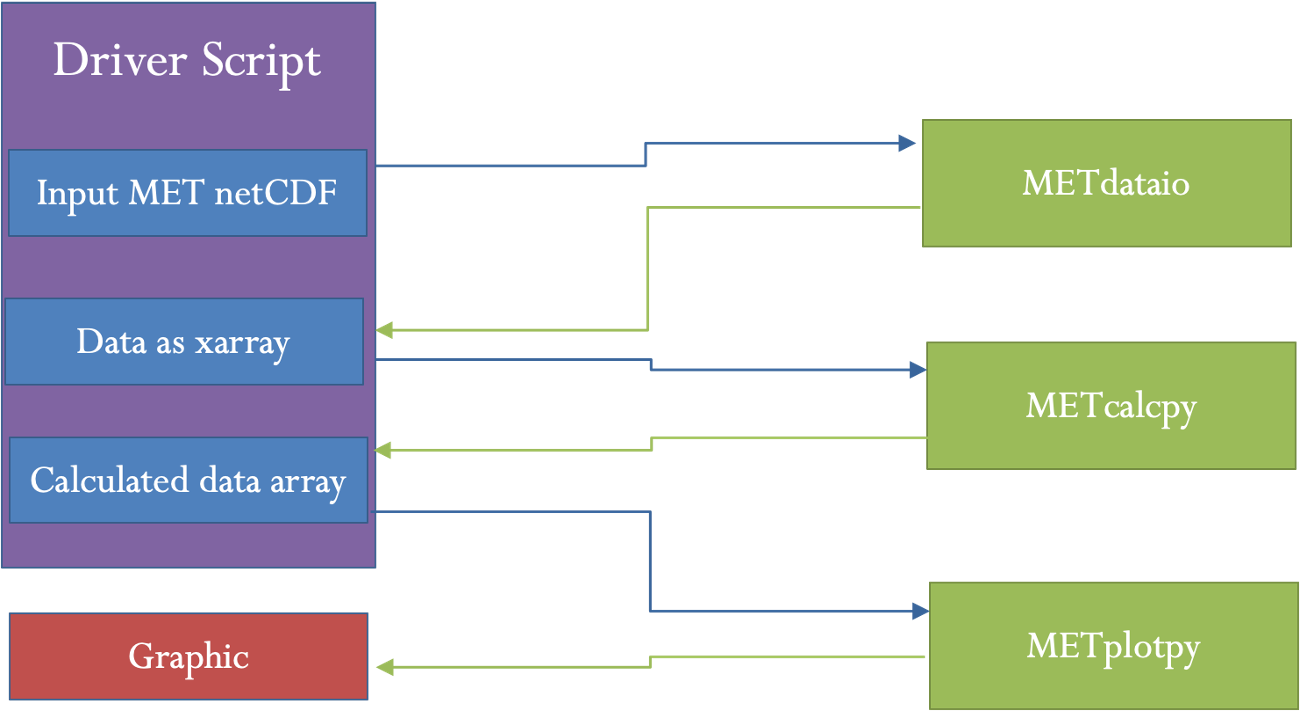
Basic Information on UserScripts
A UserScript generates user defined commands that are run from a METplus configuration file. Running a command from a METplus configuration file (as opposed to using a command line) has added benefits. These include access to METplus timing controls and filename templates. Additionally, running a command with a UserScript allows the user to link runs of METplus with other calculations or plotting scripts in any order. For the S2S use cases, UserScripts will typically call a driver script which then processes metrics, diagnostics, and/or graphics depending on the setup of the driver script. More information about the configuration and variables can be found in the UserScript section of the METplus User’s Guide.
Configuration Sections
Many of the S2S scripts use configuration sections. A configuration section is a part of the file following a label in the format of [my_new_label]. These sections are needed to run the same tool more than once with different settings. Configuration sections are called from the process list by adding the label in parenthesis after the tool name. More information about these can be found in the METplus User’s Guide section of instance names.
Final Considerations
Most of the S2S use cases require input information to the driver scripts. This information varies by use case and is given in the [user_env_vars] section of the configuration file. In most cases, this section contains options such as input variable names, directories, and plotting information. But some use cases have other variables that are needed as input to the calculation.
Different use cases have different python dependencies. These are listed in the use case documentation. The format of input data for these use cases can vary. Currently, METdataio can read netCDF data. However, most S2S use cases are set to use netCDF files that are in MET’s format. This can be achieved through pre-processing steps, typically as output from Regrid-Data-Plane or PCP-Combine.
Run METplus for the OMI use-case
Run METplus for the OMI use-case
Configuring the METplus OMI use case
The OLR-Based MJO Index (OMI)use case is one of the simplest S2S use cases, so we will start there. First, we will review the python dependencies to make sure these are available. Python dependencies for the OMI Use case we are going to run are listed in the External Dependencies section. For this case, we need to have numpy, netCDF4, datetime, xarray, matplotlib, scipy and pandas available.
This use case also requires the installation and correct environmental settings for METcalcpy and METplotpy. These requirements extend to having both of the respective repositories installed, as well as their corresponding _BASE environmental settings. Assuming that the instructions provided in the METdataio tutorial section have been followed, and the METcalcpy and METplotpy were installed in your ${METPLUS_TUTORIAL_DIR}, set the following commands:
export METDATAIO_BASE=${METPLUS_TUTORIAL_DIR}/metdataio/METdataio
export PYTHONPATH=$METDATAIO_BASE:$METCALCPY_BASE:$METPLOTPY_BASE
The file shows 2 PROCESS_LIST variables, one of which is commented out. The commented out version includes pre-processing steps which can take a long time to run due to the amount of data. Those pre-processing steps create daily means of outgoing longwave radiation (OLR) for the forecast data, and then regrid the observation and model OLR. In this example, we will be omitting those steps, running only the last two steps. The last two steps create a listing of EOF input files and then run the OMI computation.
In this case, creating a listing of EOF files is done in a separate step because the EOF files have different timing information than the input OLR files. Specifically, the EOF input is one file per day of the year, whereas the OMI in this case is computed across 2 years of OLR data. Settings for creating the list of files is given in the [create_eof_filelist] section. The command given in UserScript_COMMAND is irrelevant here as it does not affect the creation of the file lists.
Input variables to the OMI calculation are given in the [user_env_vars] section. The first two variables, OBS_RUN and FCST_RUN are either True or False, and tell the program whether to run model data, observations, or both. The third variable, SCRIPT_OUTPUT_BASE gives the location of the output graphics. The next variable tells the program how many observations per day are in the data. The last set of variables give information about formatting the plotting and output file names.
The information to run the OMI calculation is given in the [script_omi] section. The variables give the frequency of the run time, location of the model and observation input OLR data, the input template labels, which shouldn’t be changed and then the actual command that is run to calculate OMI. Here, the command calls the OMI driver script.
Run METplus for the OMI use case
${METPLUS_BUILD_BASE}/parm/use_cases/model_applications/s2s_mjo/UserScript_fcstGFS_obsERA_OMI.conf \
${METPLUS_TUTORIAL_DIR}/tutorial.conf \
config.OUTPUT_BASE=${METPLUS_TUTORIAL_DIR}/output/met_output/omi
The script should run and if successful, will say:
Check the output
Here you should see three directories (logs, s2s_mjo, and tmp) and the METplus configuration file.
There should be 2 plots inside this directory, fcst_OMI_comp_phase.png and obs_OMI_comp_phase.png. The graphics should match those displayed below.
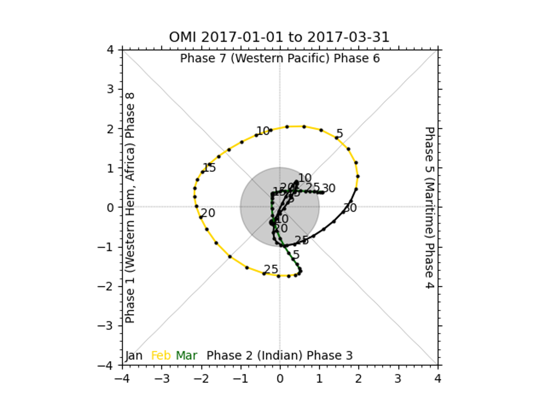
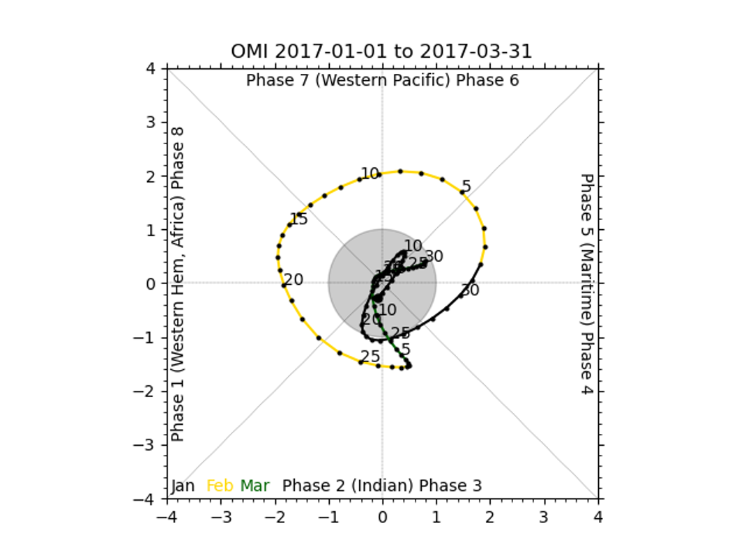
End of Session 10 and additional Exercises
End of Session 10 and additional Exercises
!!!!!!!!!!!!!!!!!!!!!!!!!!!!!!!!!!!!!!!!!!!!!!!!!!!!!!!!!!!!!!!!!!!!!!!!!!!!!!!!!!!!!!!!!!!!!!!!!!!!!!!!!!!!!!!!!!!!!!!!!!!!!!!
!!!!!!!!!!!!!!!!!!!!!!!!!!!!!!!!!!!!!!!!!!!!!!!!!!!!!!!!!!!!!!!!!!!!!!!!!!!!!!!!!!!!!!!!!!!!!!!!!!!!!!!!!!!!!!!!!!!!!!!!!!!!!!!
Run METplus for the Weather Regime use case
Background on the Weather Regime Use-Case:
The weather regime use case is more complicated than the OMI use case for several reasons. The first is that the use case has more pre-processing steps. The second is that the weather regime calculation has several steps. Specifically, it has three calculation steps and three optional output graphics for both the model and observations. Lastly, the use case calls Stat-Analysis on the output to create statistics. It uses 500mb height over December, January, and February to compute patterns for weather regime classification.
Configure the Weather Regime Use-Case:
To configure the weather regime use case, first check the python dependencies in the online User's Guide. The required python packages are numpy, netCDF4, datetime, pylab, scipy, sklearn, eofs, and matplotlib.
cd ${METPLUS_TUTORIAL_DIR}/output/met_output/weather_regime
The file shows 2 PROCESS_LIST variables, one of which is commented out. The commented out version includes pre-processing steps which can take a long time to run due to the amount of data. Here there are 2 pre-processing steps, regridding and creating daily means on the observations. The last three steps run the weather regime calculation and Stat-Analysis twice.
Input variables to the OMI calculation are given in the [user_env_vars] section. The first two variables, FCST_STEPS and OBS_STEPS are lists of the steps in each calculation that should be performed for the model and observation data. There are four calculation steps, ELBOW, EOF, KMEANS, and TIMEFREQ. The first two, ELBOW and EOF, can be omitted or run. The last step, TIMEFREQ has to be run after KMEANS. Additionally, the plotting for each step can only be run if the step is run. For example, PLOTEOF can only be run after EOF is run. In this example, all steps and plotting are turned on.
The third variable, SCRIPT_OUTPUT_BASE gives the location of the output graphics. The next variables, NUM_SEASONS and DAYS_PER_SEASON tell the code how many years of data are being input, and how many days are in each year respectively. The current setup uses data from December, January, and February of each year across 17 years. OBS_WR_VAR and FCST_WR_VAR give the names of the observation and model variables in their files. The following 11 variables control settings to the calculation including the number of weather regimes to classify, the number of clusters to use, and the frequency to use in the TIMEFREQ step. Finally, the last variables control output, including the format of the file listing the weather regime classification for each day and settings for the various plots created.
The information to run the Weather Regime calculation is given in the [script_wr] section. The variables give the frequency of the run time, location of the model and observation input 500mb height data, the input template labels, which shouldn’t be changed and then the actual command that is run. Here, the command calls the Weather Regime driver script. The last two sections [sanal_wrclass] and [sanal_wrfreq] contain the settings for running Stat-Analysis on the output weather regime classification and time frequency. These runs will not work if the KMEANS and TIMEFREQ steps are not run on both model and observation data. They produce multi category contingency table statistics on the weather regime classification and continuous statistics on the time frequency.
Run METplus for the Weather Regime use case:
${METPLUS_BUILD_BASE}/parm/use_cases/model_applications/s2s_mid_lat/UserScript_fcstGFS_obsERA_WeatherRegime.conf \
${METPLUS_TUTORIAL_DIR}/tutorial.conf \
config.OUTPUT_BASE=${METPLUS_TUTORIAL_DIR}/output/met_output/weather_regime
The script should run and if successful, will say:
Check the output:
In the ${METPLUS_TUTORIAL_DIR}/output/met_output/weather_regime directory, you should see three directories (logs, s2s_mid_lat, and tmp) and the METplus configuration file. Inside the s2s_mid_lat directory, there should be another directory, UserScript_fcstGFS_obsERA_WeatherRegime, that contains four files and two directories. The mpr directory contains output matched pair files for the weather regime classification and time frequency. The plots directory contains eight output plots, fcst_elbow.png fcst_eof.png fcst_freq.png fcst_kmeans.png obs_elbow.png obs_eof.png obs_freq.png obs_kmeans.png. Finally, there are two types of text output files. Fcst_weather_regime_class.txt and obs_weather_regime_class.txt contain text output where each day is classified into one of the six weather regime patterns. The other two files, GFS_ERA_WRClass_240000L_MCTS.stat and GFS_ERA_WRClass_240000L_MCTS.stat, contain output from stat analysis comparing the model and observation weather regime classification and time frequencies.
Session 11: METplus Cloud
Session 11: METplus Cloud
METplus Practical Session 11
This session will cover two METplus feature relative use cases.
Prerequisites: Accessing a guided tutorial EC2 instance
Running the tutorial in the cloud requires a cloud instance. Currently we are only supporting Amazon Web Services tutorial instances.
echo ${METPLUS_TUTORIAL_DIR}
echo ${METPLUS_BUILD_BASE}
echo ${MET_BUILD_BASE}
echo ${METPLUS_DATA}
ls ${METPLUS_TUTORIAL_DIR}
ls ${METPLUS_BUILD_BASE}
ls ${MET_BUILD_BASE}
ls ${METPLUS_DATA}
METPLUS_TUTORIAL_DIR is the location of all of your tutorial work, including configuration files, output data, and any other notes you'd like to keep.
METPLUS_BUILD_BASE is the full path to the METplus installation (/path/to/METplus-X.Y)
MET_BUILD_BASE is the full path to the MET installation (/path/to/met-X.Y)
METPLUS_DATA is the location of the sample test data directory
which point_stat
which run_metplus.py
If you don't see the full path to script from the shared installation, please set it. It should look the same as the output from this command:
echo ${METPLUS_BUILD_BASE}/ush/run_metplus.py
ls ${METPLUS_BUILD_BASE}/ush/run_metplus.py
If more information is needed see the instructions in Session 1 for more information.
The next section describes how to create your own EC2 instance and is optional
Create Your Own EC2 instance
Create Your Own EC2 instance
Create Your Own METplus EC2 Instance
You can also create your own EC2 instance if you have access to your own AWS account and space.
In the community AMIs tab there will be a list of prior and current METplus tutorials.
You should see a screen similar to the one below.
You should create a name that is descriptive and unique like METplus 5.0 <Your Name>.
Pre Filled Fields:
AMI from catalog – METplus 5.0 Tutorial
Instance type – t2.microo
Configure storage – 24 GIB gp2
fields should all be populated and not necessary to change
Fields To Edit:
The Key pair field needs to be chosen. You will have already set up a key pair when you created your AWS space which is out of the scope of this tutorial.
The Network settings field area can be used as is but we suggest changing the
Allow SSH traffic from:
This will limit access to this EC2 instance from much smaller subset than the entire internet.
The right hand column should have a summary of the choices you made above.
Once launched you will see a screen similar to below.
There are now two ways to get the ip address to your currently running EC2 instance.
Something similar to the image below should pop up and your ip address should be listed.
You may now connect to your EC2 instance the same way as you would if you were given an ip by the tutorial manager.
(content)
Tutorial Survey
Tutorial Survey
METplus Tutorial Survey
Thank you for your time and attention. We really enjoyed teaching you about METplus.
Please take some time to fill out the METplus Tutorial Survey to suggest improvements!
If you have more questions in your use of METplus, please:
- Refer to the MET and METplus Documentation.
- Refer to the MET Online Tutorial.
- Refer to the Known Issues Section for each release.
- Use a search engine to search for met_help followed by your question, issue, or error message.
- Browse through the MET-Help email archive.
- Open a Discussions question for help from METplus staff and community.
Now go out there and Verify!