Review the physics suites
You will run two experiments with the SCM, showing the differences between all supported physics suites for a given case based on the Tropical Warm Pool – International Cloud Experiment (TWP-ICE) field campaign. Let’s first take a look at the composition of the physics suites and then at how the case is set up.
Navigate to the directory where the Suite Definition Files (SDFs) are stored and see what is available:
ls
Peruse the files and notice the XML format, paying attention to the key elements: suite (with name attribute), group, subcycle, scheme.
You will find primary and interstitial schemes. All suites share many common elements, including interstitial schemes that are required to prepare data for schemes and calculate diagnostics.
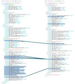
As an example, the differences between the GFS_v16 suite (an approximation of the physics used for the GFS version 16 release) and the WoFS_v0 suite (a prototype for the operational implementation of NOAA's Warn-on-Forecast System) is shown below.
Q: What are some parameterizations used in suite WoFS_v0 that are not used in suite GFS_v16?
A: Coupling of subgridscale cloudiness and RRTMG radiation scheme (sgscloud_radpre and sgscloud_radpost), the Mellow-Yamada-Nakanishi-Niino (MYNN) surface layer (mynnsfc_wrapper) and planetary boundary layer (mynnedmf_wrapper) schemes. Also note that the GFS_v16 invokes a deep convective parameterization (samfdeepcnv), while suite WoFS_v0 does not. For this reason, suite WoFS_v0 is best suited for convective-allowing models.
Review the case configuration namelists and case input data file
Now navigate to the directory where case setup namelists are stored to see what you are going to run.
ls
Look at twpice.nml to see what kinds of information are required to set up an experiment.
Each case also has a NetCDF file in DEPHY format associated with it (determined by the case_name variable) that contains the initial conditions and forcing data for the case. Take a look at one of the files to see what kind of information is expected:
There are scalar variables (single values relevant for the simulation), initial condition variables (function of vertical level only), and forcing variables (function of time and/or vertical level). Note that not all forcing variables are required to be non-zero. Additionally, there are global attributes which define the forcing type for the case.
Run the SCM
Now that you have an idea of what the physics suites contain and how to set up cases, you can run the SCM.
The following commands will get you in the bin directory and run the SCM for the TWP-ICE case using all six supported suites.
Note: if you are using a Docker container, add -d at the end of the following command
Upon a successful run, the screen output should say that the runs completed successfully and the following subdirectories will be created in $SCM_WORK/ccpp-scm/scm/run/, each of them with a log file and results in NetCDF format in file output.nc:
output_twpice_SCM_GFS_v16, output_twpice_SCM_GFS_v16_RRTMGP, output_twpice_SCM_GFS_v17_p8_ugwpv1, output_twpice_SCM_HRRR_gf, and output_twpice_SCM_WoFS_v0
Any standard NetCDF file viewing or analysis tools may be used to examine the output file (ncdump, ncview, Python, etc).
Analyze the SCM results
The output directory for each case is controlled by its case configuration namelist. For this exercise, a directory containing the output for each integration is placed in the $SCM_WORK/ccpp-scm/scm/run/ directory. Inspect that the output directories now contain a populated output.nc file.
At this point, you use whatever plotting tools you wish to examine the output. For this course, we will use the basic Python scripts that are included in the repository. The main script is called scm_analysis.py and expects a configuration file as an argument. The configuration file specifies which output files to read, which variables to plot, and how to do so.
Set up the python environment needed to run the analysis script. First create the environment using a YAML file (only once) and activate the environment using conda.
conda env create -f environment-scm_analysis.yml
conda activate env_scm_analysis
Change into the following directory:
Copy Python plotting module needed for tutorial:
Run the following to generate plots for the TWP-ICE case:
Note: if you are using a Docker container, add -d at the end of the following command
You will notice some harmless messages pertaining to “Missing variables”, which are just meant to alert the user that some suites do not have certain types of parameterizations. Therefore, tendencies for those types of parameterizations are set to zero.
The script creates a new subdirectory within the
$SCM_WORK/ccpp-scm/scm/run/ directory called plots_twpice_all_suites
Change into that directory using the command
For docker, this directory is /home/plots_twpice_all_suites/comp/active. This is also mounted outside of the container, so you can exit the container and view the output files on your home file system in the directory $OUT_DIR/plots_twpice_all_suites/comp/active.
This directory contains various plot files in PDF format. Open the files and inspect the various plots such as the precipitation time series and the mean profiles of water vapor specific humidity, cloud water mixing ratio, temperature, and temperature tendencies due to forcing and physics processes.
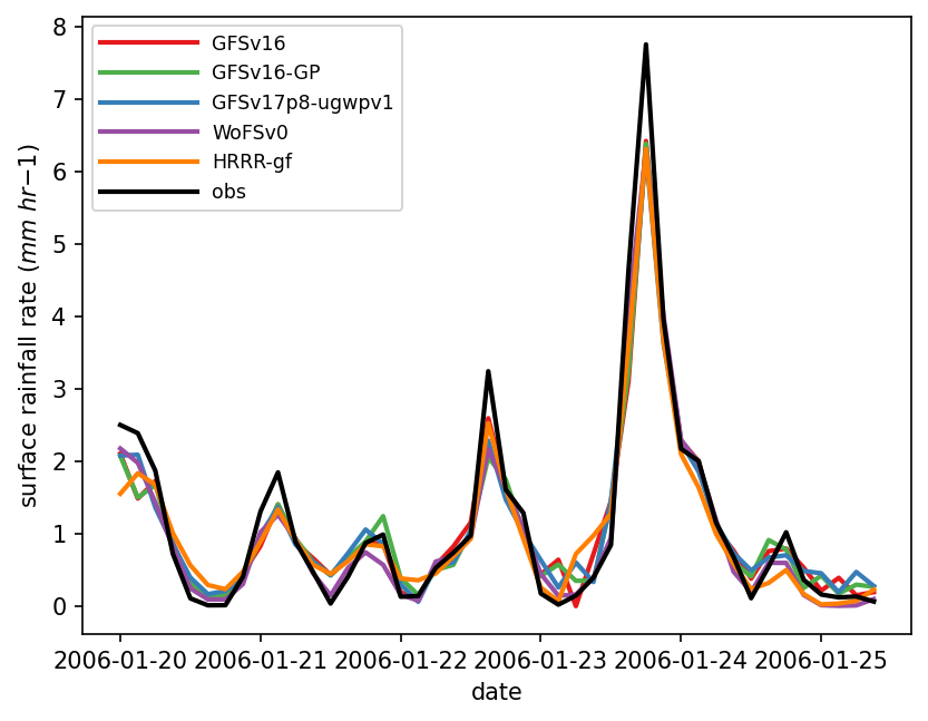
Q: Examine the prediction of precipitation in file time_series_tprcp_rate_accum.pdf. Would you say that the rain rate is well predicted in the SCM simulations?

A: All supported suites reasonably predict the evolution of rain rate as a function of time and the results for all suites are similar, indicating that, for this variable, the commonality of forcing is a stronger factor in determining the results than the differences among suites. However, it should be noted that none of the suites capture the magnitude of the largest four precipitation events.
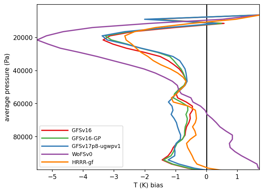
Q: Examine the profiles of temperature bias in file profiles_bias_T.pdf. In the lower troposphere (between the surface and 600 hPa), which suite(s) have a positive bias and which have a negative bias? In absolute terms, which suite has the highest bias in the lower troposphere?

A: In the lower atmosphere, suite WoFS_v0 have a positive bias (that is, it is too warm compared to observations), while all other suites have a negative bias (that is, are too cold compared to observations). In the middle atmosphere, all suites have a negative temperature bias. Suite WoFS_v0 has the largest absolute bias, which reaches -5 K.
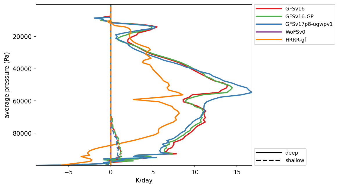
Q: Look at the tendencies due to deep and shallow convection in file profiles_mean_multi_conv_tendencies.pdf. Considering all suites, at approximately which level do the deep convective tendencies peak? And the shallow convection tendencies? Why are the convective tendencies for suite WoFS_v0 zero?

A: The deep convective scheme represents cumulus clouds that span the entire troposphere and their tendencies peak at approximately 500 hPa. The shallow convective scheme represents clouds at the top of the planetary boundary layer, with maximum tendencies at approximately 950 hPa .Suite WoFs_v0 does not produce any convective tendencies since it does not include a convective scheme because it is targeted for convective-allowing resolutions.
Q: Since it does not include a convective parameterization, is it appropriate to use suite WoFS_v0 for the SCM TWP-ICE case?
A: No, suite WoFS_v0 is included with the SCM as-is for research purposes but it is not expected to produce reasonable results for the TWP-ICE case or other CCPP SCM cases involving deep convection. This is because forcing for existing cases assumes a horizontal scale for which deep convection is subgrid-scale and is expected to be parameterized. The WoFS_v0 suite was designed for use in simulations with horizontal scale small enough not to need a deep convection parameterization active, and it does not contain a deep convective scheme. For suite WoFS_v0 to produce reasonable results with the SCM, the forcing would have to be modified to account for deep convection.
