Create a new CCPP suite, re-run the SCM, and inspect the output
In this exercise you will learn how to create a new suite and use it with the SCM. A new suite can have many different levels of sophistication. Here we will explore the simplest case, which is to add an existing CCPP physics scheme to an existing suite. In particular, we will create a modified version of the WoFS_v0 suite that contains a convective parameterization, in this case the Simplified Arakawa Schubert (SAS) scheme. One might find it useful to employ a convective parameterization (CP) when the model grid is too coarse to explicitly allow convection and when using a SCM with a forcing dataset that represents an average over a large area (such as the datasets distributed with CCPP v7.0.0).
Note that no effort has been made to optimize the inter-parameterization communication in this new suite (for example, how microphysics and convection exchange information). This new suite is offered as a technical exercise only and its results should be interpreted with caution. If you want to learn more about creating suites, read the chapter on constructing suites in the CCPP Technical Documentation as it describes how Suite Definition Files (SDFs) are constructed.
This exercise has four steps:
- Create a New Suite Definition File for Suite SCM_WoFS_v0_sas
- Prepare the Namelist File for the New Suite
- Rebuild the SCM
- Run the SCM and Inspect the Output
Step 1: Create a New Suite Definition File for suite SCM_WoFS_v0_sas
You will create a new SDF based on the SCM_WoFS_v0, but with the scale-aware SAS cumulus scheme. Note that interstitial schemes must also be added.
cp suite_SCM_WoFS_v0.xml suite_SCM_WoFS_v0_sas.xml
Edit ccpp/suites/suite_SCM_WoFS_v0_sas.xml and
- Change the suite name to “SCM_WoFS_v0_sas”
- Add the scale-aware SAS deep and shallow cumulus schemes, the associated scheme/generic interstitial schemes, and the convective cloud cover diagnostic scheme to the “physics” group. The schemes you need to add are listed in bold below. You can also copy the new SDF instead of creating your own.
- Please note that the order of schemes within groups of a suite definition file is the order in which they will be executed. In this case, the placement of the schemes follows the placement of convective schemes from other GFS-based suites. In particular, deep convection precedes shallow convection and both need to appear in the time-split section of the “slow physics” part of the suite and before the microphysics scheme is called. Decisions about the order of schemes in general are guided by many factors related to physics-dynamics coupling, including numerical stability, and should be considered carefully. For example, one of the considerations should be to understand the “data flow” within a suite for each variable used within the added schemes, e.g. when/where the variables are modified in pre-existing schemes. This can be achieved by examining the variables’ Fortran “intents” in the pre-existing schemes’ metadata.
The suite name SCM_WoFS_v0_sas is listed below with the necessary additions highlighted in bold.
<suite name="SCM_WoFS_v0_sas" version="1">
<!-- <init></init> -->
<group name="time_vary">
<subcycle loop="1">
<scheme>GFS_time_vary_pre</scheme>
<scheme>GFS_rrtmg_setup</scheme>
<scheme>GFS_rad_time_vary</scheme>
<scheme>GFS_phys_time_vary</scheme>
</subcycle>
</group>
<group name="radiation">
<subcycle loop="1">
<scheme>GFS_suite_interstitial_rad_reset</scheme>
<scheme>sgscloud_radpre</scheme>
<scheme>GFS_rrtmg_pre</scheme>
<scheme>GFS_radiation_surface</scheme>
<scheme>rad_sw_pre</scheme>
<scheme>rrtmg_sw</scheme>
<scheme>rrtmg_sw_post</scheme>
<scheme>rrtmg_lw</scheme>
<scheme>sgscloud_radpost</scheme>
<scheme>rrtmg_lw_post</scheme>
<scheme>GFS_rrtmg_post</scheme>
</subcycle>
</group>
<group name="physics">
<subcycle loop="1">
<scheme>GFS_suite_interstitial_phys_reset</scheme>
<scheme>GFS_suite_stateout_reset</scheme>
<scheme>get_prs_fv3</scheme>
<scheme>GFS_suite_interstitial_1</scheme>
<scheme>GFS_surface_generic_pre</scheme>
<scheme>GFS_surface_composites_pre</scheme>
<scheme>dcyc2t3</scheme>
<scheme>GFS_surface_composites_inter</scheme>
<scheme>GFS_suite_interstitial_2</scheme>
</subcycle>
<!-- Surface iteration loop -->
<subcycle loop="2">
<scheme>mynnsfc_wrapper</scheme>
<scheme>GFS_surface_loop_control_part1</scheme>
<scheme>sfc_nst_pre</scheme>
<scheme>sfc_nst</scheme>
<scheme>sfc_nst_post</scheme>
<scheme>lsm_noah</scheme>
<scheme>sfc_sice</scheme>
<scheme>GFS_surface_loop_control_part2</scheme>
</subcycle>
<!-- End of surface iteration loop -->
<subcycle loop="1">
<scheme>GFS_surface_composites_post</scheme>
<scheme>sfc_diag</scheme>
<scheme>sfc_diag_post</scheme>
<scheme>GFS_surface_generic_post</scheme>
<scheme>mynnedmf_wrapper</scheme>
<scheme>GFS_GWD_generic_pre</scheme>
<scheme>cires_ugwp</scheme>
<scheme>cires_ugwp_post</scheme>
<scheme>GFS_GWD_generic_post</scheme>
<scheme>GFS_suite_stateout_update</scheme>
<scheme>h2ophys</scheme>
<scheme>get_phi_fv3</scheme>
<scheme>GFS_DCNV_generic_pre</scheme>
<scheme>samfdeepcnv</scheme>
<scheme>GFS_DCNV_generic_post</scheme>
<scheme>GFS_SCNV_generic_pre</scheme>
<scheme>samfshalcnv</scheme>
<scheme>GFS_SCNV_generic_post</scheme>
<scheme>cnvc90</scheme>
<scheme>GFS_MP_generic_pre</scheme>
<scheme>mp_nssl</scheme>
<scheme>GFS_MP_generic_post</scheme>
<scheme>maximum_hourly_diagnostics</scheme>
<scheme>GFS_physics_post</scheme>
</subcycle>
</group>
<!-- <finalize></finalize> -->
</suite>
Note: If you don’t want to type, you can copy a pre-generated SDF into place:
The detailed explanation of each primary physics scheme can be found in the CCPP Scientific Documentation. A short explanation of each scheme is below:
Step 2: Prepare the Namelist File for the New Suite
We will use the default WoFS_v0 namelist input file to create the namelist file for the new suite:
cp input_WoFS_v0.nml input_WoFS_v0_sas.nml
Next, edit file input_WoFS_v0_sas.nml and modify the following namelist options to conform with the deep/shallow saSAS cumulus schemes in the SDF file :
shal_cnv = .true.
do_deep = .true.
imfdeepcnv = 2
imfshalcnv = 2
Check the Description of Physics Namelist Options for information.
Note: If you don’t want to type, you can copy a pre-generated namelist into place:
Step 3: Rebuild the SCM
Now follow these commands to rebuild the SCM with the new suite included:
cmake ../src -DCCPP_SUITES=ALL
make -j4
In addition to defining a SDF for a new suite, which only contains information about which schemes are used, one also needs to define parameters needed by the schemes in the suite (namelist file) as well as which tracers (tracer file) the SCM should carry that a given physics suite expects. There are two ways to provide this information at runtime.
- The first way is by giving command line arguments to the run script. For the namelist file, specify it with -n namelist_file.nml (assuming that the namelist file is in $SCM_WORK/ccpp-scm/ccpp/physics_namelists). For the tracer file, specify it with -t tracer_file.txt (assuming the tracer file is in $SCM_WORK/ccpp-scm/scm/etc/tracer_config).
- The second way is to define default namelist and tracer configuration files associated with the new suite in the $SCM_WORK/ccpp-scm/scm/src/suite_info.py file, where a Python list is created containing default information for the SDFs.
If you are planning on using a new suite more than just for testing purposes, it makes sense to use the second method so that you don’t have to continually use the -n and -t command line arguments when using the new suite to run the SCM.
If you try to run the SCM using a new suite and don’t specify a namelist and a tracer configuration file using either method, the run script will generate a fatal error.
For the purpose of this tutorial, you will add new default values for the new suite to make your life easier, option 2. Edit $SCM_WORK/ccpp-scm/scm/src/suite_info.py to add default namelist and tracer files associated with two suites that we will create in this tutorial (the second suite has yet to be discussed, but let’s add it now for expediency):
suite_list.append(suite('SCM_GFS_v16', 'tracers_GFS_v16.txt', 'input_GFS_v16.nml', 600.0, 1800.0, True ))
suite_list.append(suite('SCM_GFS_v17_p8', 'tracers_GFS_v17_p8.txt', 'input_GFS_v17_p8.nml', 600.0, 600.0, True ))
suite_list.append(suite('SCM_RAP', 'tracers_RAP.txt', 'input_RAP.nml', 600.0, 600.0 , True ))
suite_list.append(suite('SCM_RRFS_v1beta', 'tracers_RRFS_v1beta.txt', 'input_RRFS_v1beta.nml', 600.0, 600.0 , True ))
suite_list.append(suite('SCM_WoFS_v0', 'tracers_WoFS_v0.txt', 'input_WoFS_v0.nml', 600.0, 600.0 , True ))
suite_list.append(suite('SCM_HRRR', 'tracers_HRRR.txt', 'input_HRRR.nml', 600.0, 600.0 , True ))
suite_list.append(suite('SCM_WoFS_v0_sas', 'tracers_WoFS_v0.txt', 'input_WoFS_v0_sas.nml', 600.0, 600.0 , False))
suite_list.append(suite('SCM_WoFS_v0_sas_sfcmod', 'tracers_WoFS_v0.txt', 'input_WoFS_v0_sas.nml', 600.0, 600.0 , False))
Note: If you don’t want to type, you can copy pre-generated files into place:
Step 4: Run the Model and Inspect Output
Execute the following command to run the SCM for the TWP-ICE case using the new suite. Note that you don’t need to specify a tracer or namelist file since default ones now exist for this new suite.
Note: if you are using a Docker container, add -d at the end of the command
Upon completion of build, the following subdirectory will be created with a log file and results in NetCDF format in file output.nc:
$SCM_WORK/ccpp-scm/scm/run/output_twpice_SCM_WoFS_v0_sas
In order to generate graphics, first prepare a configuration file for the plotting script using the commands below.
Change into the following directory:
cp plot_configs/twpice_all_suites.ini plot_configs/twpice_scm_tutorial.ini
Edit plot_configs/twpice_scm_tutorial.ini. Since we only want to check how the scale-aware SAS scheme impacts the default WoFS_v0 suite, simply list the two suites in the first two lines of the file. Note that the second line defines the labels of the lines in the output plots and the third line defines the output directory for the plots.
scm_datasets_labels = WoFSv0, WoFSv0_sas
plot_dir = plots_twpice_WoFSv0_sas/
Note: If you don’t want to type, you can copy over a pre-generated plot configuration file:
Change into the following directory:
ln -s $SCM_WORK/ccpp-scm/scm/etc/scripts/plot_configs/twpice_scm_tutorial.ini twpice_scm_tutorial.ini
Create the plots with the new suite with the command below.
Note: if you are using a Docker container, add -d at the end of the command
The script creates a new subdirectory within the $SCM_WORK/ccpp-scm/scm/run/ directory called plots_twpice_WoFSv0_sas/comp/active and places the graphics in there. Open the files and inspect the various plots for changes introduced by adding a convective parameterization.
Inspect the SCM Results
Q: Examine the prediction of precipitation in file time_series_tprcp_rate_accum.pdf. How does the new suite change the precipitation?
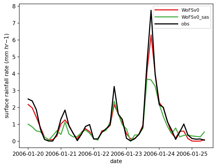
A: The time series of precipitation shows that WoFS_v0 with or without saSAS deep and shallow schemes produces similar results.
Q: Examine the profiles of temperature bias in file profiles_bias_T.pdf. How does adding a convective parameterization affect the vertical distribution of temperature bias?
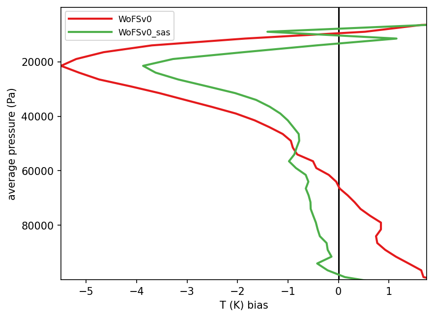
A: It is interesting to see that, when a cumulus scheme is added, the positive temperature bias below 600 hPa is adjusted to -1 K and the negative bias around the 200 hPa is adjusted to -3.5 K, which is similar to the bias of other physics suites designed for applications in coarser grid spacing, as seen in the previous exercise.