Add a new variable to a CCPP-compliant scheme
Adding a New Variable
In this section, we will explore how to pass a new variable onto an existing scheme. The surface latent and sensible heat fluxes will be adjusted in scheme fix_sys_bias_sfc to be time-dependent using the existing variable solhr (time in hours after 00 UTC at the current timestep). The surface fluxes will now only be modified between the hours of 20:30 and 8:30 UTC, which correspond to the hours of 6:00 AM and 6:00 PM local time in Darwin, Australia, where this case is located.
Step 1: Add Time Dependency to the fix_sys_bias_sfc_time Scheme
Edit file $SCM_WORK/ccpp-scm/ccpp/physics/physics/fix_sys_bias_sfc.F90 and add solhr to the argument list for subroutine fix_sys_bias_sfc_run:
Then declare solhr as a real variable:
Next, add the time-dependent surface flux modification using an if statement between the CCPP error message handling and the do loop:
A metadata entry should be added to the table for subroutine fix_sys_bias_sfc_run in file $SCM_WORK/ccpp-scm/ccpp/physics/physics/fix_sys_bias_sfc.meta.
standard_name = air_temperature_at_surface_adjacent_layer
long_name = mean temperature at lowest model layer
units = K
dimensions = (horizontal_loop_extent)
type = real
kind = kind_phys
intent = in
[solhr]
standard_name = forecast_utc_hour
long_name = time in hours after 00z at the current timestep
units = h
dimensions = ()
type = real
kind = kind_phys
intent = in
[hflx_r]
...
Note: If you don’t want to type, you can copy over completed versions of these files:
cp $SCM_WORK/tutorial_files/add_new_variable/fix_sys_bias_sfc.meta $SCM_WORK/ccpp-scm/ccpp/physics/physics/SFC_Layer/MYNN
Since solhr is an existing variable, you do not need to modify the host model. Additionally, no changes are needed in the SDF or in the prebuild script since you are simply modifying a scheme and not adding a new scheme. You can proceed to rebuilding the SCM.
Step 2: Build the Executable, Run the Model, and Inspect the Output
Issue these commands to rebuild the SCM executable:
cmake ../src -DCCPP_SUITES=ALL
make -j4
In order to avoid overwriting the output produced in exercise “Add a new scheme”, first rename the output directory:
The following command will run the SCM for the TWP-ICE case using suite WoFS_v0_sas_sfcmod with scheme fix_sys_bias_sfc modified to use variable solhr:
Note: if you are using a Docker container, add -d at the end of the command
Upon completion of the run, the following subdirectory will be created, with a log file and results in NetCDF format in file output.nc:
$SCM_WORK/ccpp-scm/scm/run/output_twpice_SCM_WoFS_v0_sas_sfcmod
To visualize the results, edit file $SCM_WORK/ccpp-scm/scm/etc/scripts/plot_configs/twpice_scm_tutorial.ini and add the new test directory name and label name to the first two lines:
output_twpice_WSAS_sfcmod/output.nc, output_twpice_SCM_WoFS_v0_sas_sfcmod/output.nc
scm_datasets_labels = WoFSv0_sas,WoFSv0_sas_sfcmod,WoFSv0_sas_sfcmod_time
plot_dir = plots_twpice_WoFSv0_sas_sfcmod_time/
Note: If you don’t want to type, you can copy over a pre-generated plot configuration file:
Change into the following directory:
Next, run the following command to generate plots for the last three exercises in this tutorial.
Note: if you are using a Docker container, add -d at the end of the command
The script creates a new subdirectory within the $SCM_WORK/ccpp-scm/scm/run/ directory called plots_twpice_R_sas_sfcmod_time/comp/active
Inspect the Results
Q: Examine the surface latent heat flux and the surface sensible heat flux in files time_series_lhf.pdf and time_series_shf.pdf, respectively. How does the latent heat flux differ from the previous exercise?
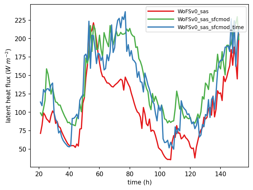
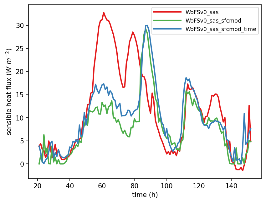
A: Instead of adding 40 W m-2 to the latent heat flux throughout the simulation, the latent heat flux value was modified only between the hours of 6 AM and 6 PM local time to mimic the observed diurnal cycle feature.
Q: Examine the temperature bias and the specific humidity bias in files profiles_bias_T.pdf and profiles_bias_qv.pdf, respectively. How are the temperature and moisture profiles affected by the surface latent heat flux modification?
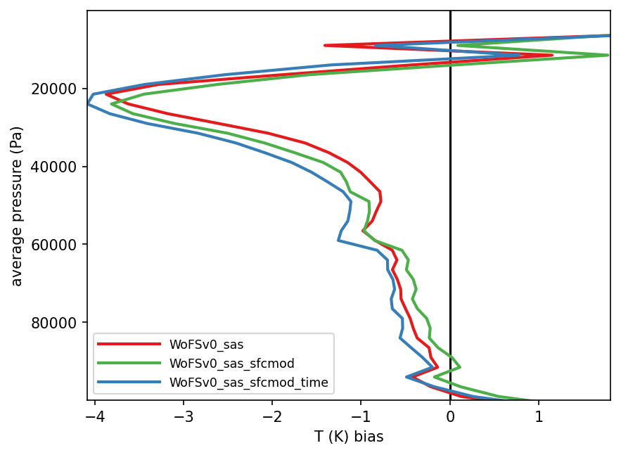

A: Even though we effectively added more energy to the atmosphere, the net effect in the T and q profiles are either neutral or show an increase in negative bias. This points out that physics suites have complicated non-linear interactions and that it is often possible to get unexpected results. This also points to the utility of studying physics in a SCM context, where one at least has a chance at understanding the mechanisms when only dealing with one column and are excluding interactions/feedbacks due the presence and advection from surrounding columns.