NWP Containers Online Tutorial
NWP Containers Online TutorialEnd-to-End NWP Container Online Tutorial
This online tutorial describes step-by-step instructions on how to obtain, build, and run each containerized component using Docker.
(Updated 09/2022)
How to get help
Please post questions or comments about this tutorial to the GitHub Discussions forum for the DTC NWP Containers project.
Using the Online Tutorial
Throughout this tutorial, the following conventions are used:
- Bold font is used for directory and filenames and occasionally to simply indicate emphasis.
- The following formatting is used for things to be typed on the command line:
- Use the forward arrow " > " at the bottom of each page to continue.
- Use the backward arrow " < " to return to the previous page.
Look for tips and hints.
Start the Online Tutorial
Throughout this tutorial, you will have to type several commands on the command line and edit settings in several files. Those commands are displayed in this tutorial in such a way that it is easy to copy and paste them directly from the webpage. You are encouraged to do so to avoid typing mistakes and speed your progress through the tutorial.
Introduction
IntroductionSimplifying end-to-end numerical modeling using software containers
Software systems require substantial set-up to get all the necessary code, including external libraries, compiled on a specific platform. Recently, the concept of containers has been gaining popularity because they allow for software systems to be bundled (including operating system, libraries, code, and executables) and provided directly to users, eliminating possible frustrations with up-front system setup.
Using containers allows for efficient, lightweight, secure, and self-contained systems. Everything required to make a piece of software run is packaged into isolated containers, ready for development, shipment, and deployment. Using containers guarantees that software will always run the same, regardless of where it is deployed.
Ultimately, containers substantially reduce the spin-up time of setting up and compiling software systems and promote greater efficiency in getting to the end goal of producing model output and statistical analyses.
Advantages to using containers for NWP
- Reduces spin-up time to build necessary code components
- Highly portable
- Use in cloud computing
- Easily sharable with other collaborators
- Easy to replicate procedures and results
Who can benefit from using NWP containers?
- Graduate and undergraduate students
- University faculty
- Researchers
- Tutorial participants
Tutorial format
Throughout this tutorial, code blocks in BOLD white text with a black background should be copied from your browser and pasted on the command line.
echo "Let's Get Started"
Platform Options
Platform OptionsContainer software
While many software containerization platforms exist, two are supported for running the end-to-end containerized NWP system: Docker or Singularity.
Docker |
Singularity |
|---|---|
|
Docker was the first container platform explored by this project and, thus, has been tested robustly across local machines and on the cloud (AWS). Using Docker, the end-to-end containerized NWP system described here is fully functional on a local machine or on AWS. A few disadvantages to the Docker software are that root permissions are required to install and update, and it requires additional tools to run across multiple nodes, which are not needed nor supported for this particular application.
|
Singularity is also an option for running all but the final component (METviewer) of the end-to-end containerized NWP system by converting Docker images on Dockerhub to Singularity image files. Similar to Docker, installing and updating Singularity software requires root permissions. A few advantages to Singularity are that it was designed for High Performance Computing (HPC) platforms and can more efficiently run on multiple nodes on certain platforms. The functionality to run METviewer using Singularity is still a work in progress, so if there is a desire to create verification plots from the MET output, it will be necessary to use Docker for this step at this time.
|
Compute platform
There are two recommended methods for running this tutorial; follow the instructions that you find most useful below.
Running on a local machine |
Running on a cloud computing platform |
|---|---|
|
If you have access to a Linux/Unix based machine–whether a laptop, desktop, or compute cluster–it is likely that you will be able to run this entire tutorial on that machine. Click here for instructions for "Running On A Local Machine" |
This tutorial can also be run on the Amazon Web Services (AWS) cloud compute platform. We provide a pre-built image which should have all the software necessary for running the tutorial. Cloud computing costs will be incurred. Click here for instructions for "Running in the Cloud" |
Running on a local machine
Running on a local machineRunning tutorial on a local machine
To run this tutorial on a local machine, you will need to have access to a number of different utilities/software packages:
- A terminal or terminal emulator for running standard Linux/Unix commands (ls, cd, mkdir, etc.)
- untar and gzip
- A text editor such as vim, emacs, or nano
- Docker (see below)
- git (optional; see below)
More detailed instructions for certain requirements can be found below:
Installing container software
In order to run the NWP containers described in this tutorial, a containerization software (Docker or Singularity) will need to be available on your machine. To download and install the desired version software compatible with your system, please visit
- Docker: https://www.docker.com/get-started
- Singularity: https://sylabs.io/guides/3.6/user-guide/quick_start.html
In order to install Docker or Singularity on your machine, you will be required to have root access privileges. Once the software has been installed, Singularity can be run without root privileges, with a few exceptions.
Docker and Singularity are updated on a regular basis; we recommended applying all available updates.
Git version control software
The scripts and Dockerfiles used during this tutorial live in a git repository. You can download a project .tar file from the Github website, or, if you wish, you can clone the repository using git software. Specific instructions for doing this will be found on subsequent pages.
If you would like to use git and it is not installed git on your machine, please visit https://git-scm.com to learn more. Prior to using git for the first time, you will need to configure your git environment. For example:
git config --global user.email user@email.com
Running on the cloud
Running on the cloudAmazon Web Services (AWS)
This tutorial has been designed for use on Amazon Web Services (AWS) cloud computing. Other cloud computing platforms may be used, but the instructions below will have to be modified accordingly.
In order to complete this tutorial on AWS, one must launch an EC2 instance that is configured with the proper environment, software, and library dependencies. In addition to a number of library dependencies, the primary software and utilities include:
- Docker (required)
- Singularity (required)
- wgrib2
- ncview
- ImageMagick
Building the proper AWS environment can be achieved in two ways:
| Launch an EC2 instance from the DTC maintained AMI | Build & configure the EC2 instance from scratch |
|---|---|
| An AMI (Amazon Machine Image) is simply a saved copy of the EC2 environment that can be used to launch a new EC2 Instance with all of these software and tools pre-installed, allowing the user to quickly launch the proper EC2 Instance and begin the tutorial. Read more about AMIs here. The DTC maintains and provides a public AMI called "dtc-utility-base-env_v4.1.0" that contains all of these required tools. | Steps are provided to install all of the required software and tools from scratch. The user may then create an AMI if they choose, and may additionally choose to include tutorial specific content (e.g. data, container images, scripts) in their AMI as well, depending on user needs. |
Follow the instructions below for the preferred choice of acquiring the AWS environment:
Below you will find steps to create an EC2 Instance from the DTC AMI called "dtc-utility-base-env_v4.1.0", and login to your new instance from a terminal window.
See AWS documentation for more information
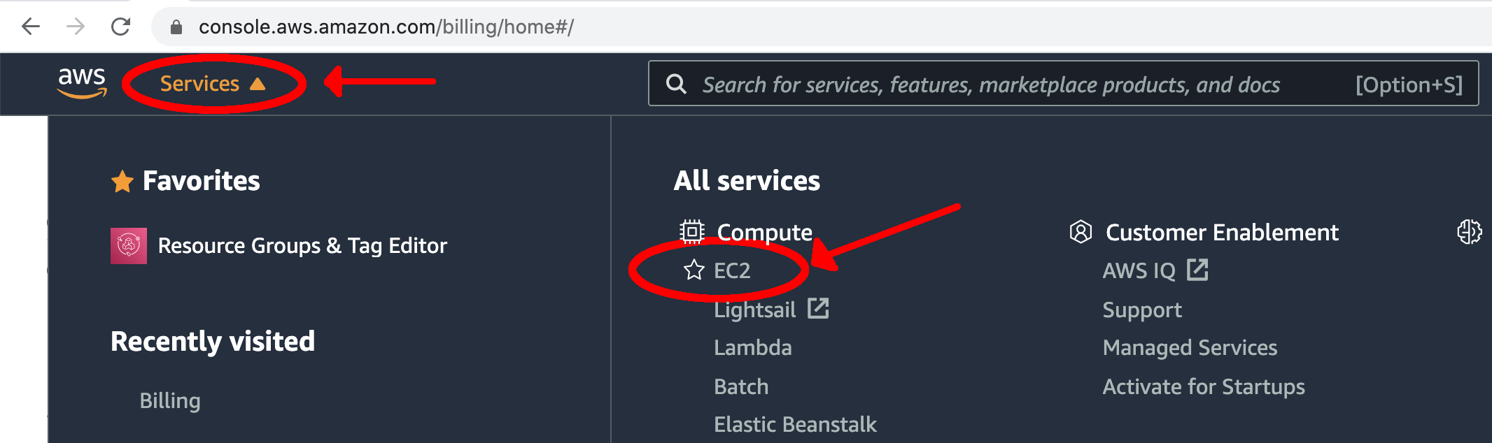
- Navigate to Amazon’s Elastic Compute Cloud (EC2) Management Console by clicking on the "Services" tab at the top. Under the "Compute" section, select "EC2".
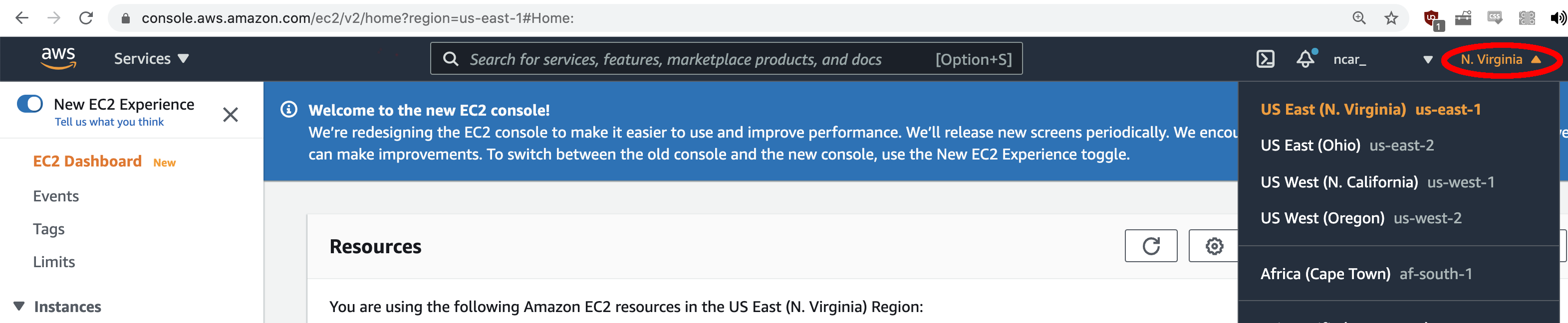
- Determine what region you are running under by looking in the top right corner of the screen. To use the DTC AMI, you need to use the "N. Virginia" region. If this is not what you see, use the drop-down arrow and select the "US East (N. Virginia)" region.
For this tutorial, you can use an environment that has already been established for you: an Amazon Machine Image (AMI).
- Click the "AMIs" link on the left side "EC2 Dashboard"
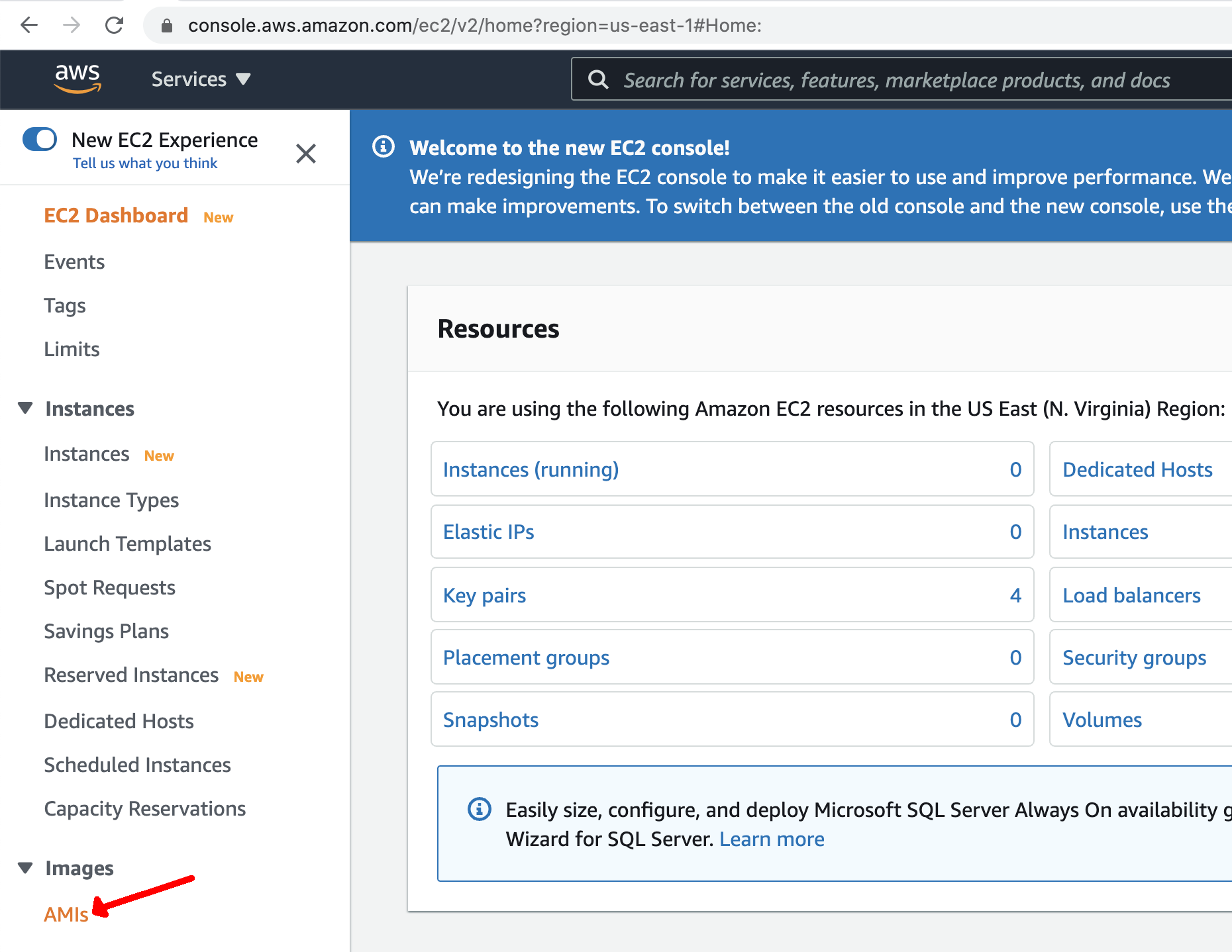
You will initially not see any AMIs listed, since you do not own any images.
- Select "Public Images" from the dropdown as shown.
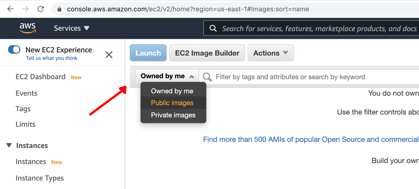
- In the search bar, enter in the name of the DTC AMI: "dtc-utility-base-env_v4.1.0" and press enter.
- Select the resulting AMI from the list window.
- Once selected, click the blue "Launch" button at the top of the page
After launching the AMI, the next step is to configure the instance prior to using it.
- From the "Filter by" dropdown list, select the "c5" option (a "compute-optimized" instance; see this page for more info on AWS instance types) to see a smaller list of possible selections.
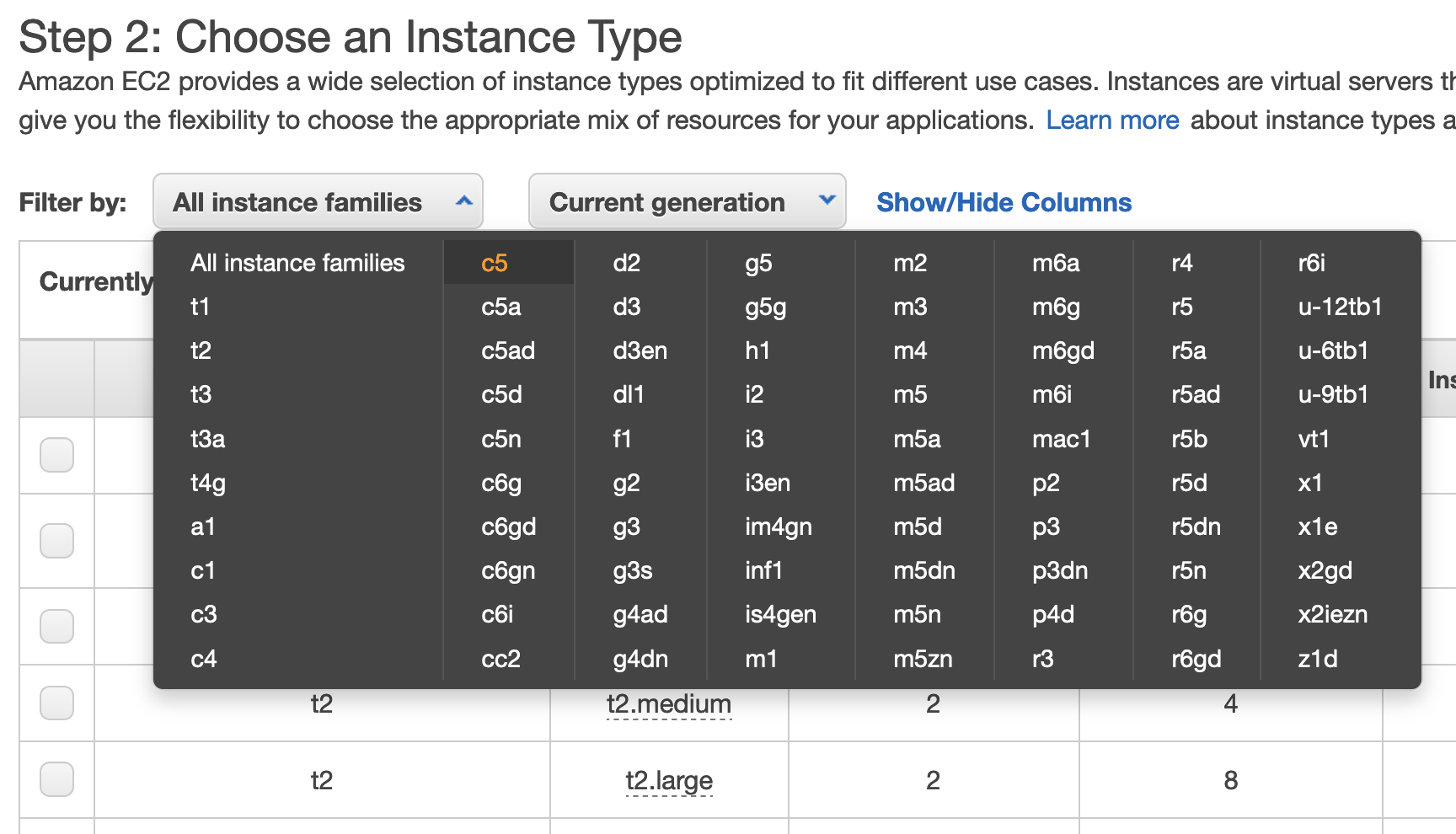
- Scroll down and click the box next to the "c5.4xlarge" instance type and click the "Next: Configure Instance Details" button on the bottom right of the page.
- There is no need to further configure the instance details on the next page so simply click the button the bottom right of the page for "Next: Add Storage"
- If the storage size has not already been increased, change the storage from the default of 8 to 60 Gb and click the "Next: Add Tags" button on the bottom right of the page.
- Add a personal tag to identify what instance is yours.
- Select the blue link in the middle of the page that says "click to add a Name tag". This is a key-value pair where key=Name and value=your_personal_nametag
- On the next page the key will automatically be set to "Name" (leave this as is) and you simply assign a name of your choice to the Value in the second box. The value can be set to anything you will recognize and is unlikely to be used by anyone else. Note, it is not recommended to use any spaces in your name.
- NOTE: The key should literally be called "Name"; do not change the text in the left box
- Click the "Next: Configure Security Group" button on the bottom right of the page.
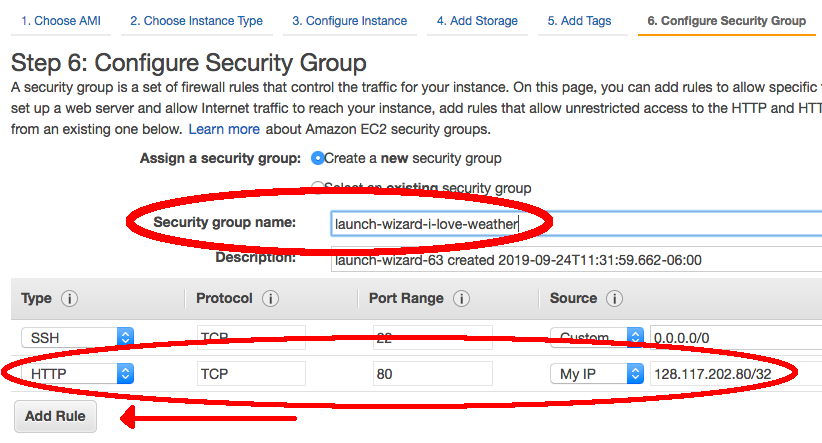
- Amazon requires us to set a unique security group name for each AWS instance. We will also need to set some rules in order to properly set up access to visualize verification output with the METviewer GUI. These steps will both be done on the "Configure Security Group" page.
- The field "Security group name" will be filled in with an automated value. If other tutorial users are attempting to launch an instance with this same automated value, it will fail, so you should replace the given value with any unique group name you desire.
- Select the button on the left hand side that says "Add Rule". Under the drop down menu, select "HTTP". The port range for HTTP is 80.
- Note: Rules with source of 0.0.0.0/0 allow all IP addresses to access your instance. You can modify setting security group rules to allow access from known IP addresses only by clicking the "Custom" drop down menu and selecting "My IP".
- Click the blue "Review and Launch" button at the bottom of the page to continue.
- You can review the selected configuration settings and select the blue "Launch" button in the bottom right corner.
- It will be necessary to create an ssh key pair to allow for SSH access into your instance.
- In the first drop down box, choose "create a new key pair".
- In the second box for the key pair name, choose any name you’d like but make sure it does not include any spaces. (e.g., your_name-aws-ssh)
- Click the "Download Key Pair" button and the key pair will be placed in your local Downloads directory, named: name_you_chose.pem (Note, Some systems will add .txt to the end of the *.pem file name so the file may actually be named name_you_chose.pem.txt)
Windows users: please review Windows information sheet
- To access your instance running in the cloud you first need to set up your ssh access from your remote system
- Open a terminal window and create a new directory to access your AWS cloud instance
mkdir ~/AWS - Go into the new directory and then move your *.pem file into it and change the permissions of the file
cd ~/AWS
mv ~/Downloads/name_you_chose.pem .
chmod 600 name_you_chose.pem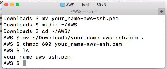
- Open a terminal window and create a new directory to access your AWS cloud instance
- Finally, back in your browser window:
- click "Launch Instances"
- click the blue "View Instances" button on the bottom right corner of the next page.
- Look for the instance with the name you gave it. As soon as you see a green dot and "Running" under the "Instance State" column, your instance is ready to use!
- You will need to obtain your IPV4 Public IP from the AWS "Active Instances" web page. This can be found from your AWS instances page as shown below:
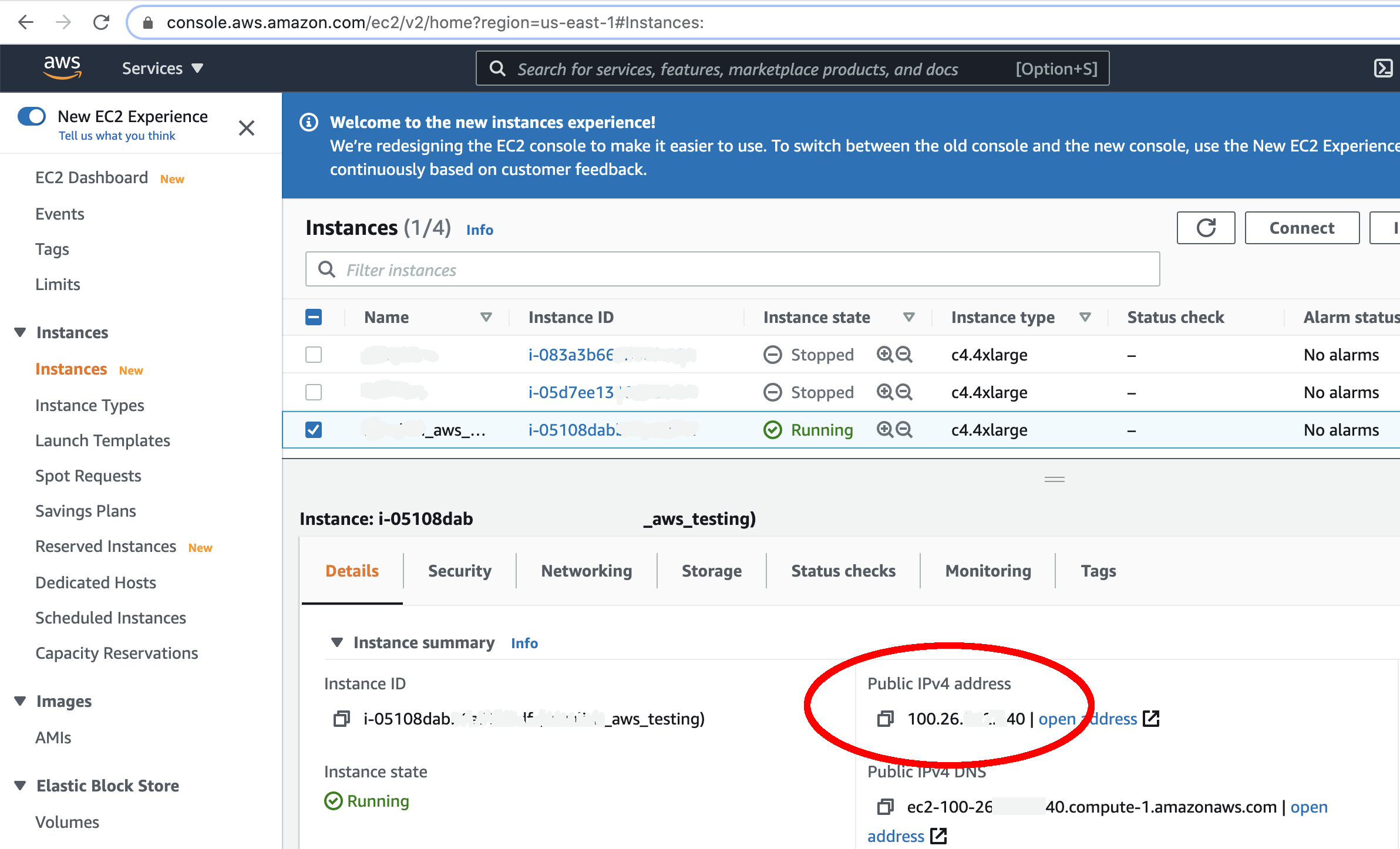
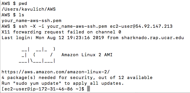
- From your newly created AWS directory, ssh into your instance. (Windows users: please review Windows information sheet)
ssh -X -i name_you_chose.pem ec2-user@IPV4_public_IPOR on a mac, change the “X” to a “Y”:
ssh -Y -i name_you_chose.pem ec2-user@IPV4_public_IP - The IPV4 public IP is something that is unique to your particular instance. If you stop/re-start your instance, this public IP will be different each time.
- Feel free to open multiple terminals and log into your instance (using the same credentials) several times if you so desire.
- From this point on, you will mostly be working in your terminal window; however, you may occasionally need to look back at the AWS web page, so be sure to keep the AWS console open in your browser.
- Once you are in your instance from the terminal window you should see the following set-up:
Below you will find the steps necessary to create an EC2 instance and install the libraries and software required to complete this tutorial, along with a number of helpful utilities to inspect output files created as part of this tutorial.
After completing these steps, you can create your own AMI for future use if you choose. You may also choose to complete the tutorial, or portions of the tutorial, and then create an AMI. For example, suppose you want to include the container images, tutorial repository contents, and input data in your AMI for future use. Simply complete the above steps to create the base environment and software, then complete the tutorial menu items: Repository, Downloading Input Data, and NWP Containers. Then create the AMI. Note that this is a completely customizable procedure and may benefit from some experience/knowledge with AWS AMIs and familiarity with this tutorial first.
Information on creating an AMI of your own can be found in the AWS documentation.
- Select: Amazon Linux 2 AMI (HVM), SSD Volume Type (64 bit/x86)
- Select: C5.4xlarge
- Select: Change storage to 60 GB
- Configure Security Group: Add rule for HTTP (Set Source to MyIP)
(use your own pem file and public IP address from the instance you launched in step 1):
mkdir /home/ec2-user/utilities
Install packages
sudo yum install -y libX11-devel.x86_64 Xaw3d-devel.x86_64 libpng-devel.x86_64 libcurl-devel.x86_64 expat-devel.x86_64 ksh.x86_64
Compile HDF5 from source
wget https://support.hdfgroup.org/ftp/HDF5/releases/hdf5-1.10/hdf5-1.10.5/src/hdf5-1.10.5.tar.gz
tar -xvzf hdf5-1.10.5.tar.gz; rm hdf5-1.10.5.tar.gz
cd hdf5-1.10.5
./configure --with-zlib=/usr/lib64 --prefix=/home/ec2-user/utilities
make install
Compile netCDF from source
wget ftp://ftp.unidata.ucar.edu/pub/netcdf/netcdf-c-4.7.1.tar.gz
tar -xvzf netcdf-c-4.7.1.tar.gz; rm netcdf-c-4.7.1.tar.gz
cd netcdf-c-4.7.1
./configure --prefix=/home/ec2-user/utilities CPPFLAGS=-I/home/ec2-user/utilities/include LDFLAGS=-L/home/ec2-user/utilities/lib
make install
Compile UDUNITS from source
wget ftp://ftp.unidata.ucar.edu/pub/udunits/udunits-2.2.28.tar.gz
tar -xvzf udunits-2.2.28.tar.gz; rm udunits-2.2.28.tar.gz
cd udunits-2.2.28
./configure -prefix=/home/ec2-user/utilities
make install
Compile ncview from source
wget ftp://cirrus.ucsd.edu/pub/ncview/ncview-2.1.7.tar.gz
tar -xvzf ncview-2.1.7.tar.gz; rm ncview-2.1.7.tar.gz
cd ncview-2.1.7
sudo ln -sf /usr/include/X11/Xaw3d /usr/include/X11/Xaw
./configure --with-nc-config=/home/ec2-user/utilities/bin/nc-config --prefix=/home/ec2-user/utilities --with-udunits2_incdir=/home/ec2-user/utilities/include --with-udunits2_libdir=/home/ec2-user/utilities/lib
make install
Install ImageMagick and x11
sudo yum install -y ImageMagick ImageMagick-devel
Install docker
sudo service docker start
sudo usermod -a -G docker ec2-user
Start Docker automatically upon instance creation
Install docker-compose
sudo chmod +x /usr/local/bin/docker-compose
- To ensure that Docker is correctly initialized, one time only you must:
- exit
- Log back in with same IP address
- (DO NOT terminate the instance)
ssh -Y -i file.pem ec2-user@pubIPaddress
Install wgrib2
wget ftp://ftp.cpc.ncep.noaa.gov/wd51we/wgrib2/wgrib2.tgz
tar -xvzf wgrib2.tgz; rm wgrib2.tgz
cd grib2
export CC=`which gcc`
export FC=`which gfortran`
make
make lib
Install Singularity prerequisites
sudo yum update -y
sudo yum install -y openssl-devel libuuid-devel libseccomp-devel wget squashfs-tools
export GO_VERSION=1.13 OS=linux ARCH=amd64
Install Go
sudo tar -C /usr/local -xzvf go${GO_VERSION}.${OS}-${ARCH}.tar.gz; sudo rm go${GO_VERSION}.${OS}-${ARCH}.tar.gz
echo 'export PATH=/usr/local/go/bin:$PATH' >> ~/.bashrc
source ~/.bashrc
Install Singularity
git clone https://github.com/sylabs/singularity.git
cd singularity
git checkout tags/v${SINGULARITY_VERSION}
sudo ./mconfig
sudo make -C builddir
sudo make -C builddir install
sed -i 's/^hstgo=/hstgo=\/usr\/local\/go\/bin\/go/g' mconfig
sudo ./mconfig
sudo make -C builddir
sudo make -C builddir install
Finally, you should enter your home directory and modify the .bashrc and .bash_profile files to properly set the environment each time you log in.
Edits to .bashrc are shown in bold
if [ -f /etc/bashrc ]; then
. /etc/bashrc
fi
# Uncomment the following line if you don't like systemctl's auto-paging feature:
# export SYSTEMD_PAGER=
# User specific aliases and functions
export PATH=/usr/local/go/bin:$PATH
export PROJ_DIR=/home/ec2-user
alias wgrib2="/home/ec2-user/utilities/grib2/wgrib2/wgrib2"
alias ncview="/home/ec2-user/utilities/bin/ncview"
alias ncdump="/home/ec2-user/utilities/bin/ncdump"
Additionally, you should add the following line to ~/.bash_profile:
Then, source the .bash_profile file to enable these new changes to the environment
Access AWS EC2 on Windows
Access AWS EC2 on WindowsAccessing an EC2 Instance on your Windows Machine
There are a few different ways to access a terminal-type environment on a Windows machine. Below are a few of the most common methods. Users can first create their EC2 Instance as described in the online procedures, then use one of the options below to access their instance on their Windows machine.
After downloading and installing WSL, you can access and run a native Linux environment directly on your Windows machine. In the WSL terminal window you can then run all of the Linux/Mac tutorial procedures as-is. https://docs.aws.amazon.com/AWSEC2/latest/UserGuide/WSL.html
Using PuTTY requires a user to convert their .pem key file to the PuTTY format .ppk file using the PuTTYgen application. Then use the PuTTY GUI to connect to the instance with the newly created .ppk file. This will launch a terminal window connected to your EC2 instance. https://docs.aws.amazon.com/AWSEC2/latest/UserGuide/putty.html
With MobaXTerm installed you can open a MobaXterm terminal window and connect directly using same provided instructions for Linux/Mac with your .pem file. You can also use the GUI to log into your instance as well. Examples can be found online demonstrating the GUI.
AWS Tips
AWS TipsBelow are several tips for running the NWP containers on AWS. This list will be updated as we uncover new tips and tricks!
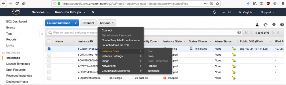
Starting, stopping, and terminating images
When you are done working but would like to save where you left off (data output, script modifications, etc.), you should stop your instance. Stopped instances do not incur usage or data transfer fees; however, you will be charged for storage on any Amazon Elastic Block Storage (EBS) volumes. If the instance state remains active, you will incur the charges.
When you no longer need an instance, including all output, file modifications, etc., you can terminate an instance. Terminating an instance will stop you from incurring anymore charges. Keep in mind that once an instance has been terminated you can not reconnect to it or restart it.
These actions can be carried out by first selecting "Instances" on the left hand side navigation bar. Next, select the instance you wish to either stop or terminate. Then, under the "Actions" button, select "Instance State" and choose your desired action.
Logging out and back into an instance
In the scenario where you need to log out or stop an instance, you can log back in and resume your work. However, you will need to reset the PROJ_DIR (Note: In the DTC private AMI, the PROJ_DIR is already set in the environment) and CASE_DIR environment variables to get your runs to work according to the instructions. Also, if you stop an instance and restart it, you will be assigned a new IPv4 Public IP that you will use when you ssh into your instance.
Transferring files to and from a local machine to an AWS instance
If you need to copy files between your local machine and AWS instance, follow these helpful examples.
Transfers to/from AWS is always initiated from your local machine/terminal window.
In the example below, we will copy namelist.wps from our local /home directory to ec2-user's /home directory. To copy files from your local machine to your instance:
In this example, we will copy wps_domain.png from ec2-user's /home directory to our local /home directory. To copy files from your instance to your local machine:
NOTE: Copying data out of an EC2 instance can incur high charges per GB, it is advised to only copy small files such as images and text files rather than large data files.
Container Software Commands and Tips
Container Software Commands and TipsThis page contains common commands and tips for Docker or Singularity (click link to jump to respective sections).
Docker
Common docker commands
Listed below are common Docker commands, some of which will be run during this tutorial. For more information on command-line interfaces and options, please visit: https://docs.docker.com/engine/reference/commandline/docker/
- Getting help:
- docker --help : lists all Docker commands
- docker run --help : lists all options for the run command
- Building or loading images:
- docker build -t my-name . : builds a Docker image from Dockerfile
- docker save my-name > my-name.tar : saves a Docker image to a tarfile
- docker load < my-name.tar.gz : loads a Docker image from a tarfile
- Listing images and containers:
- docker images : lists the images that currently exist, including the image names and ID's
- docker ps -a : lists the containers that currently exist, including the container names and ID's
- Deleting images and containers:
- docker rmi my-image-name: removes an image by name or ID
- docker rmi $(docker images -q) or docker rmi `docker images -q` : removes all existing images
- docker rm my-container-name : removes a container by name or ID
- docker rm $(docker ps -a -q) or docker rm `docker ps -aq` : removes all existing containers
- These commands can be forced with by adding -f
- Creating and running containers:
- docker run --rm -it \
--volumes-from container-name \
-v local-path:container-path \
--name my-container-name my-image-name : creates a container from an image, where:- --rm : automatically removes the container when it exits
- -it : creates an interactive shell in the container
- --volumes-from : mounts volumes from the specified container
- -v : defines a mapping between a local directory and a container directory
- --name : assigns a name to the container
- docker exec my-container-name : executes a command in a running container
- docker-compose up -d : defines and runs a multi-container Docker application
- docker run --rm -it \
Docker run commands for this tutorial
This tutorial makes use of docker run commands with several different arguments. Here is one example:
docker run --rm -it -e LOCAL_USER_ID=`id -u $USER` \
-v ${PROJ_DIR}/container-dtc-nwp/components/scripts/common:/home/scripts/common \
-v ${PROJ_DIR}/container-dtc-nwp/components/scripts/sandy_20121027:/home/scripts/case \
-v ${CASE_DIR}/wpsprd:/home/wpsprd -v ${CASE_DIR}/gsiprd:/home/gsiprd -v ${CASE_DIR}/wrfprd:/home/wrfprd \
--name run-sandy-wrf dtcenter/wps_wrf:${PROJ_VERSION} /home/scripts/common/run_wrf.ksh
The different parts of this command are detailed below:
-
docker run --rm -it
- As described above, this portion creates and runs a container from an image, creates an interactive shell, and automatically removes the container when finished
-
-e LOCAL_USER_ID=`id -u $USER`
- The `-e` flag sets an environment variable in the interactive shell. In this case, our containers have been built with a so-called "entrypoint" that automatically runs a script on execution that sets the UID within the container to the value of the LOCAL_USER_ID variable. In this case, we are using the command `id -u $USER` to output the UID of the user outside the container. This means that the UID outside the container will be the same as the UID inside the container, ensuring that any files created inside the container can be read outside the container, and vice versa
-
-v ${PROJ_DIR}/container-dtc-nwp/components/scripts/common:/home/scripts/common
- As described above, the `-v` flag mounts the directory ${PROJ_DIR}/container-dtc-nwp/components/scripts/common outside of the container to the location /home/scripts/common within the container. The other -v commands do the same
-
--name run-dtc-nwp-derecho
- Assigns the name "run-dtc-nwp-derecho" to the running container
-
dtcenter/wps_wrf:${PROJ_VERSION}
- The "${PROJ_VERSION}" tag of image "dtcenter/wps_wrf" will be used to create the container. This should be something like "4.0.0", and will have been set in the "Set Up Environment" step for each case
-
/home/scripts/common/run_wrf.ksh
- Finally, once the container is created (and the entrypoint script is run), the script "/home/scripts/common/run_wrf.ksh" (in the container's directory structure) will be run, which will set up the local environment and input files and run the WRF executable.
Common Docker problems
Docker is a complicated system, and will occasionally give you unintuitive or even confusing error messages. Here are a few that we have run into and the solutions that have worked for us:
-
Problem: When mounting a local directory, inside the container it is owned by root, and we can not read or write any files in that directory
-
Solution: Always specify the full path when mounting directories into your container.
-
When "bind mounting" a local directory into your container, you must specify a full path (e.g. /home/user/my_data_directory) rather than a relative path (e.g. my_data_directory). We are not exactly sure why this is the case, but we have reliably reproduced and solved this error many times in this way.
-
-
Problem: Log files for executables run with MPI feature large numbers of similar error messages:
-
Read -1, expected 682428, errno = 1
Read -1, expected 283272, errno = 1
Read -1, expected 20808, errno = 1
Read -1, expected 8160, errno = 1
Read -1, expected 390504, errno = 1
Read -1, expected 162096, errno = 1 -
etc. etc.
-
These errors are harmless, but their inclusion can mask the actual useful information in the log files, and in long WRF runs can cause the log files to swell to unmanageable sizes.
-
-
Solution: Add the flag "--cap-add=SYS_PTRACE" to your docker run command
-
For example:
docker run --cap-add=SYS_PTRACE --rm -it -e LOCAL_USER_ID=`id -u $USER` -v ${PROJ_DIR}/container-dtc-nwp/components/scripts/common:/home/scripts/common -v ${CASE_DIR}/wrfprd:/home/wrfprd -v ${CASE_DIR}/wpsprd:/home/wpsprd -v ${PROJ_DIR}/container-dtc-nwp/components/scripts/derecho_20120629:/home/scripts/case --name run-dtc-nwp-derecho dtcenter/wps_wrf:${PROJ_VERSION} /home/scripts/common/run_wrf.ksh -np 8
-
Singularity
Common Singularity commands
Listed below are common Singularity commands, some of which will be run during this tutorial. For more information on command-line interfaces and options, please visit: https://sylabs.io/guides/3.7/user-guide/quick_start.html#overview-of-the-singularity-interface
If a problem occurs during the building of a singularity image from dockerhub (for example, running out of disk space) it can result in a corrupted cache for that image causing it to not run properly, even if you re-pull the container. You can clear the cache using the command:
On the Cheyenne supercomputer, downloading and converting a singularity image file from Dockerhub may use too many resources and result in you being kicked off a login node. To avoid this, you can run an interactive job on the Casper machine using the `execdav` command (this example requests a 4-core job for 90 minutes)
Common Singularity problems
As with Docker, Singularity is a complicated system, and will occasionally give you unintuitive or even confusing error messages. Here are a few that we have run into and the solutions that have worked for us:
-
Problem: When running a singularity container, I get the following error at the end:
-
INFO: Cleaning up image...
ERROR: failed to delete container image tempDir /some_directory/tmp/rootfs-979715833: unlinkat /some_directory/tmp/rootfs-979715833/root/root/.tcshrc: permission denied
-
-
Solution: This problem is due to temporary files created on disk when running Singularity outside of "sandbox" mode. They can be safely ignored
Repository
RepositoryFirst we will set up some directories and variables that we will use to run this tutorial. Navigate to the top-level experiment directory (where you will run the experiments in this tutorial) and set the environment variable PROJ_DIR as this base directory. This directory must be in a location that has at least 25 Gb of storage space available in order for the tutorial to work. Your commands will be different depending on the shell you are using, for example:
| For tcsh: | For bash or ksh: |
|---|---|
|
# or your top-level experiment dir
mkdir -p /home/ec2-user cd /home/ec2-user setenv PROJ_DIR `pwd` setenv PROJ_VERSION 4.1.0
|
# or your top-level experiment dir
mkdir -p /home/ec2-user cd /home/ec2-user export PROJ_DIR=`pwd` export PROJ_VERSION="4.1.0"
|
Next, you should obtain the scripts and dockerfiles from the NWP container repository using Git.
Obtain the end-to-end container project from GitHub
The end-to-end NWP container project repository can be found at:
https://github.com/NCAR/container-dtc-nwp
Obtain the code base by copying and pasting the entire following command:
The contents of container-dtc-nwp contain scripts and files to build the images/containers and run this tutorial.
Downloading Input Data
Downloading Input DataStatic and initialization data
Two types of datasets will need to be available on your system to run WPS and WRF. The first is a static geographical dataset that is interpolated to the model domain defined by the geogrid program in WPS. To reduce the necessary size footprint, only a subset of coarse static geographical data is provided. The second is model initialization data that is also processed through WPS and the real.exe program to supply initial and lateral boundary condition information at the start and during the model integration.
Additionally, a tarball for GSI data assimilation will be needed, containing CRTM coefficient files. And a tarball containing shapefiles is needed for running the Python plotting scripts.
Information on how to download data is detailed in this tutorial. If a user has access to datasets on their local machine, they can also point to that data when running the containers.
Please follow the appropriate section below that fits your needs.
NOTE: If you do not plan on running all the test cases, you can omit downloading all of the model input data and only download those cases you are interested in. All cases require the CRTM and WPS_GEOG data, however.
For other platforms, you can download this data from the DTC website:
mkdir data/
cd data/
curl -SL https://dtcenter.ucar.edu/dfiles/container_nwp_tutorial/tar_files/container-dtc-nwp-derechodata_20120629.tar.gz | tar zxC .
curl -SL https://dtcenter.ucar.edu/dfiles/container_nwp_tutorial/tar_files/container-dtc-nwp-sandydata_20121027.tar.gz | tar zxC .
curl -SL https://dtcenter.ucar.edu/dfiles/container_nwp_tutorial/tar_files/container-dtc-nwp-snowdata_20160123.tar.gz | tar zxC .
curl -SL https://dtcenter.ucar.edu/dfiles/container_nwp_tutorial/tar_files/CRTM_v2.3.0.tar.gz | tar zxC .
curl -SL https://dtcenter.ucar.edu/dfiles/container_nwp_tutorial/tar_files/wps_geog.tar.gz | tar zxC .
curl -SL https://dtcenter.ucar.edu/dfiles/container_nwp_tutorial/tar_files/shapefiles.tar.gz | tar zxC .
You should now see all the data you need to run the three cases in this directory, grouped into five directories:
drwxr-xr-x 35 user admin 1120 May 13 22:52 WPS_GEOG/
drwxr-xr-x 3 user admin 96 Nov 12 2018 model_data/
drwxr-xr-x 4 user admin 128 Nov 12 2018 obs_data/
drwxr-xr-x 3 user admin 96 Sep 10 2021 shapefiles/
For users of the NCAR Cheyenne machine, the input data has been staged on disk for you to copy. Make a directory named "data" and unpack the data there:
mkdir data/
cd data/
| tcsh | bash |
|---|---|
|
foreach f (/glade/p/ral/jntp/NWP_containers/*.tar.gz)
tar -xf "$f" end |
for f in /glade/p/ral/jntp/NWP_containers/*.tar.gz; do tar -xf "$f"; done
|
You should now see all the data you need to run the three cases in this directory:
| ls -al | ||||||
| drwxr-xr-x | 3 | user | ral | 4096 | Jul 21 2020 | gsi |
| drwxrwxr-x | 3 | user | ral | 4096 | Nov 12 2018 | model_data |
| drwxrwxr-x | 3 | user | ral | 4096 | Nov 12 2018 | obs_data |
| drwxrwxr-x | 4 | user | ral | 4096 | Sep 10 2021 | shapefiles |
| drwxrwxr-x | 35 | user | ral | 4096 | May 13 16:52 | WPS_GEOG |
Sandy Data
Sandy Data jwolff Mon, 03/25/2019 - 09:43For the Hurricane Sandy case example, Global Forecast System (GFS) forecast files initialized at 12 UTC on 20121027 out 48 hours in 3-hr increments are provided. Prepbufr files from the North American Data Assimilation System (NDAS) are provided for point verification and data assimilation, and Stage II precipitation analyses are included for gridded verification purposes.
There are two options for establishing the image from which the data container will be instantiated:
- Pull the image from Docker Hub
- Build the image from scratch
Please follow the appropriate section below that fits your needs.
Option 1: Pull the dtcenter/sandy image from Docker Hub
If you do not want to build the image from scratch, simply use the prebuilt image by pulling it from Docker Hub.
docker pull dtcenter/sandy
To instantiate the data container, type the following:
To see what images you have available on your system, type:
To see what containers you have running on your system, type:
Option 2: Build the dtcenter/sandy image from scratch
To access the model initialization data for the Hurricane Sandy case from the Git repository and build it from scratch, first go to your project space where you cloned the repository:
and then build an image called dtcenter/sandy:
This command goes into the case_data/sandy_20121027 directory and reads the Dockerfile directives. Please review the contents of the case_data/sandy_20121027/Dockerfile for additional information.
To instantiate the case data container, type the following:
To see what images you have available on your system, type:
To see what containers you have running on your system, type:
Snow Data
Snow Data jwolff Mon, 03/25/2019 - 09:40For the snow case example, Global Forecast System (GFS) forecast files initialized at 00 UTC on 20160123 out 24 hours in 3-hr increments are provided. Prepbufr files from the North American Data Assimilation System (NDAS) are provided for point verification and data assimilation, and MRMS precipitation analyses are included for gridded verification purposes.
There are two options for establishing the image from which the data container will be instantiated:
- Pull the image from Docker Hub
- Build the image from scratch
Please follow the appropriate section below that fits your needs.
Option 1: Pull the dtcenter/snow image from Docker Hub
If you do not want to build the image from scratch, simply use the prebuilt image by pulling it from Docker Hub.
docker pull dtcenter/snow
To instantiate the case data container, type the following:
To see what images you have available on your system, type:
To see what containers you have running on your system, type:
Option 2: Build the dtcenter/snow image from scratch
To access the model initialization data for the snow case from the Git repository and build it from scratch, first go to your project space where you cloned the repository:
and then build an image called dtcenter/snow:
This command goes into the case_data/snow_20160123 directory and reads the Dockerfile directives. Please review the contents of the case_data/snow_20160123/Dockerfile for additional information.
To instantiate the case data container, type the following:
To see what images you have available on your system, type:
To see what containers you have running on your system, type:
Derecho data
Derecho data jwolff Mon, 03/25/2019 - 09:42For the derecho case example, Global Forecast System (GFS) forecast files initialized at 12 UTC on 20120629 out 24 hours in 3-hr increments are provided. Prepbufr files from the North American Data Assimilation System (NDAS) are provided for point verification and data assimilation, and Stage II precipitation analyses are included for gridded verification purposes.
There are two options for establishing the image from which the data container will be instantiated:
- Pull the image from Docker Hub
- Build the image from scratch
Please follow the appropriate section below that fits your needs.
Option 1: Pull the prebuilt dtcenter/derecho image
If you do not want to build the image from scratch, simply use the prebuilt image by pulling it from Docker Hub.
docker pull dtcenter/derecho
To instantiate the case data container, type the following:
To see what images you have available on your system, type:
To see what containers you have running on your system, type:
Option 2: Build the dtcenter/derecho image from scratch
To access the model initialization data for the Derecho case from the Git repository and build it from scratch, first go to your project space where you cloned the repository:
and then build an image called dtcenter/derecho:
This command goes into the case_data/derecho_20120629 directory and reads the Dockerfile directives. Please review the contents of the case_data/derecho_20120629/Dockerfile for additional information.
To instantiate the case data container, type the following:
To see what images you have available on your system, type:
To see what containers you have running on your system, type:
Software Containers
Software ContainersEach component of the end-to-end NWP container system has its own software container. There are three options for establishing each image from which the software container will be instantiated:
1. Pull the image from Docker Hub
2. Build the image from scratch
3. Pull the Docker Hub image and convert it to a Singularity image
Instructions are provided for all three options. Please follow the appropriate section that fits your needs.
WPS and WRF NWP Components
WPS and WRF NWP ComponentsThe wps_wrf software container consists of two components:
- WRF Preprocessing System (WPS)
- Advanced Weather Research and Forecasting (WRF-ARW) model
There are three options for establishing the image from which the software container will be instantiated. Please follow the appropriate section below that fits your needs.
Option 1: Pull the dtcenter/wps_wrf image from Docker Hub
If you do not want to build the image from scratch, simply use the prebuilt image by pulling it from Docker Hub.
docker pull dtcenter/wps_wrf:${PROJ_VERSION}
To see what images you have available on your system, type:
Option 2: Build the dtcenter/wps_wrf image from scratch
To access the preprocessing (WPS) and model (WRF) code from the Git repository and build the image from scratch, first go to your project space where you cloned the repository:
and then build an image called dtcenter/wps_wrf:
This command goes into the wps_wrf directory and reads the Dockerfile directives. Please review the contents of the wps_wrf/Dockerfile for additional information.
To see what images you have available on your system, type:
Option 3: Pull the dtcenter/wps_wrf Docker Hub image and convert it to a Singularity image
If you are using Singularity rather than Docker, the commands are similar:
singularity pull docker://dtcenter/wps_wrf:${PROJ_VERSION}_for_singularity
Unlike Docker, Singularity does not keep track of available images in a global environment; images are stored in image files with the .sif extension. Use the `ls` command to see the image file you just downloaded
GSI data assimilation
GSI data assimilationThe GSI container will be used to perform data assimilation. There are three options for establishing the image from which the software container will be instantiated. Please follow the appropriate section below that fits your needs.
Option 1: Pull the dtcenter/gsi image from Docker Hub
If you do not want to build the image from scratch, simply use the prebuilt image by pulling it from Docker Hub.
docker pull dtcenter/gsi:${PROJ_VERSION}
To see what images you have available on your system, type:
Option 2: Build the dtcenter/gsi image from scratch
To access the GSI container from the Git repository and build the image from scratch, first go to your project space where you cloned the repository:
and then build an image called dtcenter/gsi:
This command goes into the gsi directory and reads the Dockerfile directives. Please review the contents of the gsi/Dockerfile for additional information.
To see what images you have available on your system, type:
OPTION 3: Pull the dtcenter/gsi Docker Hub image and convert it to a Singularity image
If you are using Singularity rather than Docker, the commands are similar:
singularity pull docker://dtcenter/gsi:${PROJ_VERSION}
Unlike Docker, Singularity does not keep track of available images in a global environment; images are stored in image files with the .sif extension. Use the `ls` command to see the image file you just downloaded
-rwxr-xr-x 1 ec2-user ec2-user 879349760 Sep 29 20:49 wps_wrf_${PROJ_VERSION}.sif
Unified Post Processor (UPP)
Unified Post Processor (UPP)The UPP container will be used to post process the model output. There are three options for establishing the image from which the software container will be instantiated. Please follow the appropriate section below that fits your needs.
Option 1: Pull the dtcenter/upp image from Docker Hub
If you do not want to build the image from scratch, simply use the prebuilt image by pulling it from Docker Hub.
docker pull dtcenter/upp:${PROJ_VERSION}
To see what images you have available on your system, type:
Option 2: Build the dtcenter/upp image from scratch
To access the UPP container from the Git repository and build the image from scratch, first go to your project space where you cloned the repository:
and then build an image called dtcenter/upp:
This command goes into the upp directory and reads the Dockerfile directives. Please review the contents of the upp/Dockerfile for additional information.
To see what images you have available on your system, type:
Option 3: Pull the dtcenter/upp Docker Hub image and convert it to a Singularity image
If you are using Singularity rather than Docker, the commands are similar:
singularity pull docker://dtcenter/upp:${PROJ_VERSION}
Unlike Docker, Singularity does not keep track of available images in a global environment; images are stored in image files with the .sif extension. Use the `ls` command to see the image file you just downloaded
-rwxr-xr-x 1 ec2-user ec2-user 1224183808 Sep 29 21:04 upp_${PROJ_VERSION}.sif
-rwxr-xr-x 1 ec2-user ec2-user 879349760 Sep 29 20:49 wps_wrf_${PROJ_VERSION}.sif
Python Graphics
Python GraphicsThe Python container will be used to plot model forecast fields. There are three options for establishing the image from which the software container will be instantiated. Please follow the appropriate section below that fits your needs.
Option 1: Pull the dtcenter/python image from Docker Hub
If you do not want to build the image from scratch, simply use the prebuilt image by pulling it from Docker Hub.
docker pull dtcenter/python:${PROJ_VERSION}
To see what images you have available on your system, type:
Option 2: Build the dtcenter/python image from scratch
To access the Python scripts from the Git repository and build the image from scratch, first go to your project space where you cloned the repository:
and then build an image called dtcenter/python:
This command goes into the python directory and reads the Dockerfile directives. Please review the contents of the python/Dockerfile for additional information.
To see what images you have available on your system, type:
Option 3: Pull the dtcenter/python Docker Hub image and convert it to a Singularity image
If you are using Singularity rather than Docker, the commands are similar:
singularity pull docker://dtcenter/python:${PROJ_VERSION}
Unlike Docker, Singularity does not keep track of available images in a global environment; images are stored in image files with the .sif extension. Use the `ls` command to see the image file you just downloaded
-rwxr-xr-x 1 ec2-user ec2-user 646881280 Sep 29 21:28 python_${PROJ_VERSION}.sif
-rwxr-xr-x 1 ec2-user ec2-user 1224183808 Sep 29 21:04 upp_${PROJ_VERSION}.sif
-rwxr-xr-x 1 ec2-user ec2-user 879349760 Sep 29 20:49 wps_wrf_${PROJ_VERSION}.sif
MET Verification
MET VerificationVerification of the model fields will be performed using the Model Evaluation Tools (MET) container. There are three options for establishing the image from which the software container will be instantiated. Please follow the appropriate section below that fits your needs.
Option 1: Pull the dtcenter/nwp-container-met image from Docker Hub
If you do not want to build the image from scratch, simply use the prebuilt image by pulling it from Docker Hub.
docker pull dtcenter/nwp-container-met:${PROJ_VERSION}
To see what images you have available on your system, type:
Option 2: Build the dtcenter/nwp-container-met image from scratch
To access the Model Evaluation Tools (MET) code from the Git repository and build the verification software from scratch, first go to your project space where you cloned the repository:
and then build an image called dtcenter/nwp-container-met:
This command goes into the met/MET directory and reads the Dockerfile directives. Please review the contents of the met/MET/Dockerfile for additional information.
To see what images you have available on your system, type:
Option 3: Pull the dtcenter/met Docker Hub image and convert it to a Singularity image
If you are using Singularity rather than Docker, the commands are similar:
singularity pull docker://dtcenter/nwp-container-met:${PROJ_VERSION}
Unlike Docker, Singularity does not keep track of available images in a global environment; images are stored in image files with the .sif extension. Use the `ls` command to see the image file you just downloaded
-rwxr-xr-x 1 ec2-user ec2-user 1045712896 Sep 29 21:34 nwp-container-met_${PROJ_VERSION}.sif
-rwxr-xr-x 1 ec2-user ec2-user 646881280 Sep 29 21:28 python_${PROJ_VERSION}.sif
-rwxr-xr-x 1 ec2-user ec2-user 1224183808 Sep 29 21:04 upp_${PROJ_VERSION}.sif
-rwxr-xr-x 1 ec2-user ec2-user 879349760 Sep 29 20:49 wps_wrf_${PROJ_VERSION}.sif
METviewer Database and Display
METviewer Database and DisplayOnce verification scores for each valid time have been computed in the MET container, the METviewer database can be loaded and the user interface can be launched in your web-browser to compute summary statistics and display them. There are two options for establishing the image from which the software container will be instantiated. Please follow the appropriate section below that fits your needs.
Option 1: Pull the dtcenter/metviewer image from Docker Hub
If you do not want to build the image from scratch, simply use the prebuilt image by obtaining the tar file and loading it.
docker pull dtcenter/nwp-container-metviewer:${PROJ_VERSION}
If you followed all the instructions up to this point in the tutorial, the output should look similar to this:
| REPOSITORY | TAG | IMAGE ID | CREATED | SIZE |
| dtcenter/wps_wrf | 3.5.1 | 9b2f58336cf9 | 3 hours ago | 3.22GB |
| dtcenter/nwp-container-met | 3.5.1 | 9e3d0e924a30 | 3 hours ago | 5.82GB |
| dtcenter/upp | 3.5.1 | 82276dfccbc3 | 4 hours ago | 3.36GB |
| dtcenter/nwp-container-metviewer | 3.5.1 | f2095355127f | 4 hours ago | 2.8GB |
| dtcenter/python | 3.5.1 | 7ea61e625dff | 4 hours ago | 1.28GB |
| dtcenter/gsi | 3.5.1 | c6bebdbfb674 | 5 hours ago | 2.88GB |
Option 2: Build the dtcenter/metviewer image from scratch
To access the METviewer database and display system from the Git repository and build the verification software from scratch, first go to your project space where you cloned the repository:
and then build an image called dtcenter/metviewer:
This command goes into the metviewer/METviewer directory and reads the Dockerfile directives. Please review the contents of the metviewer/METviewer/Dockerfile for additional information.
To see what images you have available on your system, type:
Option 3: Pull the dtcenter/metviewer Docker Hub image and convert it to a Singularity image
If you are using Singularity rather than Docker, the commands are similar:
singularity pull docker://dtcenter/nwp-container-metviewer-for-singularity:${PROJ_VERSION}
Unlike Docker, Singularity does not keep track of available images in a global environment; images are stored in image files with the .sif extension. Use the `ls` command to see the image file you just downloaded
-rwxr-xr-x 1 ec2-user ec2-user 1045712896 Sep 29 21:34 nwp-container-met_${PROJ_VERSION}.sif
-rwxr-xr-x 1 ec2-user ec2-user 1045712896 Sep 29 21:34 nwp-container-metviewer-for-singularity_${PROJ_VERSION}.sif
-rwxr-xr-x 1 ec2-user ec2-user 646881280 Sep 29 21:28 python_${PROJ_VERSION}.sif
-rwxr-xr-x 1 ec2-user ec2-user 1224183808 Sep 29 21:04 upp_${PROJ_VERSION}.sif
-rwxr-xr-x 1 ec2-user ec2-user 879349760 Sep 29 20:49 wps_wrf_${PROJ_VERSION}.sif
Hurricane Sandy Case (27 Oct 2012)
Hurricane Sandy Case (27 Oct 2012)Case overview
Reason for interest: Destructive hurricane
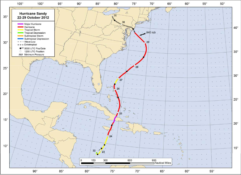
The most deadly and destructive hurricane during the 2012 Atlantic hurricane season, Hurricane Sandy was a late-season storm that developed from a tropical wave in the western Caribbean. It quickly intensified into a tropical storm and made its first landfall as a Category 1 storm over Jamaica. As the storm progressed northward, it continued to strengthen into a Category 3 storm, prior to making landfall on eastern Cuba and subsequently weakening back to a Category 1 hurricane. Sandy continued weakening to tropical-storm strength as it moved up through the Bahamas, and then began re-intensifying as it pushed northeastward parallel to the United States coastline. Ultimately, Sandy curved west-northwest, maintaining its strength as it transitioned to an extratropical cyclone just prior to coming onshore in New Jersey with hurricane force winds.
In total, more than 230 fatalities were directly or indirectly associated with Hurricane Sandy. Sandy impacted the the Caribbean, Bahamas, Bermuda, the southeastern US, Mid-Atlantic and New England states, up through eastern Canada. Sandy was blamed for $65 billion in damage in the U.S. alone, making it the fourth-costliest hurricane in U.S. history as of August 2019.
NHC Best track positions for Hurricane Sandy, 22-29 October 2012:
Observed precipitation for 192 hours (12 UTC 24 Oct - 12 UTC 1 Nov 2012) courtesy of the NWS/WPC:
Set up environment
Set up environmentSet Up Environment
To run the Hurricane Sandy case, first establish environment variables for this case study
If you have not already done so, navigate to the top-level experiment directory (where you have downloaded the container-dtc-nwp directory) and set the environment variables PROJ_DIR and PROJ_VERSION.
| tcsh | bash |
|---|---|
|
cd /home/ec2-user
setenv PROJ_DIR `pwd` setenv PROJ_VERSION 4.1.0
|
cd /home/ec2-user
export PROJ_DIR=`pwd` export PROJ_VERSION="4.1.0"
|
Then, you should set up the variables and directories for the Sandy experiment
| tcsh | bash |
|---|---|
|
setenv CASE_DIR ${PROJ_DIR}/sandy
|
export CASE_DIR=${PROJ_DIR}/sandy
|
cd ${CASE_DIR}
mkdir -p wpsprd wrfprd gsiprd postprd pythonprd metprd metviewer/mysql
Extra step for singularity users
Users of singularity containerization software will need to set a special variable for temporary files written by singularity at runtime:
| tcsh | bash |
|---|---|
|
setenv TMPDIR ${PROJ_DIR}/sandy/tmp
|
export TMPDIR=${PROJ_DIR}/sandy/tmp
|
Run NWP initialization components
Run NWP initialization componentsRun NWP Initialization Components
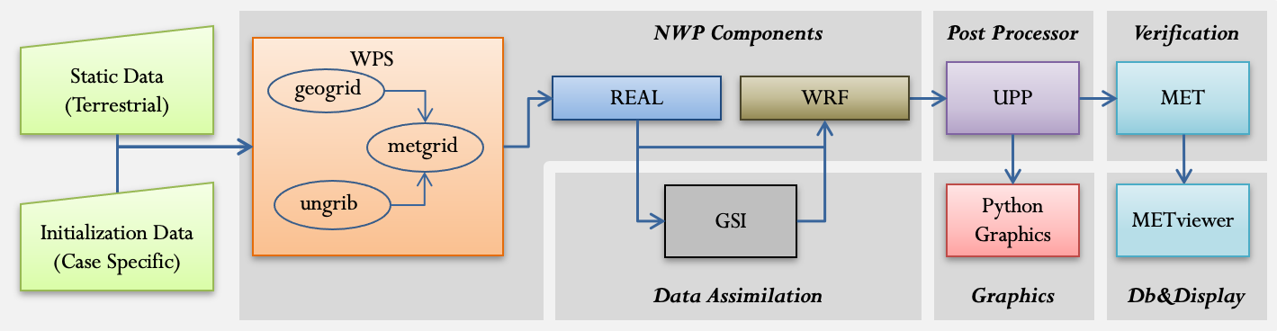
The NWP workflow process begins by creating the initial and boundary conditions for running the WRF model. This will be done in two steps using WPS (geogrid.exe, ungrib.exe, metgrid.exe) and WRF (real.exe) programs.
Initialization Data
Global Forecast System (GFS) forecast files initialized at 18 UTC on 20121027 out 48 hours in 3-hr increments are provided for this case.
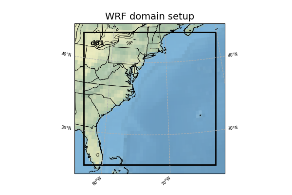
Model Domain
The WRF domain we have selected covers most of the east coast of the United States, and a portion of the northwestern Atlantic Ocean. The exact domain is shown below:
Select the appropriate container instructions for your system below:
Step One (Optional): Run Python to Create Image of Domain
A Python script has been provided to plot the computational domain that is being run for this case. If desired, run the dtcenter/python container to execute Python in docker-space using the namelist.wps in the local scripts directory, mapping the output into the local pythonprd directory.
-v ${PROJ_DIR}/container-dtc-nwp/components/scripts/common:/home/scripts/common \
-v ${PROJ_DIR}/container-dtc-nwp/components/scripts/sandy_20121027:/home/scripts/case \
-v ${PROJ_DIR}/data/shapefiles:/home/data/shapefiles \
-v ${CASE_DIR}/pythonprd:/home/pythonprd \
--name run-sandy-python dtcenter/python:${PROJ_VERSION} \
/home/scripts/common/run_python_domain.ksh
A successful completion of the Python plotting script will result in the following file in the pythonprd directory. This is the same image that is shown at the top of the page showing the model domain.
Step Two: Run WPS
Using the previously downloaded data (in ${PROJ_DIR}/data), while pointing to the namelists in the local scripts directory, run the dtcenter/wps_wrf container to run WPS in docker-space and map the output into the local wpsprd directory.
-v ${PROJ_DIR}/data/WPS_GEOG:/data/WPS_GEOG \
-v ${PROJ_DIR}/data:/data -v ${PROJ_DIR}/container-dtc-nwp/components/scripts/common:/home/scripts/common \
-v ${PROJ_DIR}/container-dtc-nwp/components/scripts/sandy_20121027:/home/scripts/case \
-v ${CASE_DIR}/wpsprd:/home/wpsprd --name run-sandy-wps dtcenter/wps_wrf:${PROJ_VERSION} \
/home/scripts/common/run_wps.ksh
Once WPS begins running, you can watch the log files being generated in another window by setting the ${CASE_DIR} environment variable and tailing the log files:
Type CTRL-C to exit the tail utility.
A successful completion of the WPS steps will result in the following files (in addition to other files) in the wpsprd directory
FILE:2012-10-27_18
FILE:2012-10-27_21
FILE:2012-10-28_00
met_em.d01.2012-10-27_18:00:00.nc
met_em.d01.2012-10-27_21:00:00.nc
met_em.d01.2012-10-28_00:00:00.nc
Step Three: Run real.exe
Using the previously downloaded data (in ${PROJ_DIR}/data), output from WPS in step one, and pointing to the namelists in the local scripts directory, run the dtcenter/wps_wrf container to this time run real.exe in docker-space and map the output into the local wrfprd directory.
-v ${PROJ_DIR}/data:/data -v ${PROJ_DIR}/container-dtc-nwp/components/scripts/common:/home/scripts/common \
-v ${PROJ_DIR}/container-dtc-nwp/components/scripts/sandy_20121027:/home/scripts/case \
-v ${CASE_DIR}/wpsprd:/home/wpsprd \
-v ${CASE_DIR}/wrfprd:/home/wrfprd --name run-sandy-real dtcenter/wps_wrf:${PROJ_VERSION} \
/home/scripts/common/run_real.ksh
The real.exe program should take less than a minute to run, but you can follow its progress as well in the wrfprd directory:
Type CTRL-C to exit the tail utility.
A successful completion of the REAL step will result in the following files (in addition to other files) in the wrfprd directory
wrfinput_d01
Step One (Optional): Run Python to Create Image of Domain
A Python script has been provided to plot the computational domain that is being run for this case. If desired, run the dtcenter/python container to execute Python in singularity-space using the namelist.wps in the local scripts directory, mapping the output into the local pythonprd directory.
A successful completion of the Python plotting script will result in the following file in the pythonprd directory. This is the same image that is shown at the top of the page showing the model domain.
Step Two: Run WPS
Using the previously downloaded data (in ${PROJ_DIR}/data), while pointing to the namelists in the local scripts directory, run the wps_wrf container to run WPS in singularity-space and map the output into the local wpsprd directory.
Once WPS begins running, you can watch the log files being generated in another window by setting the ${CASE_DIR} environment variable and tailing the log files:
Type CTRL-C to exit the tail utility.
A successful completion of the WPS steps will result in the following files (in addition to other files) in the wpsprd directory
FILE:2012-10-27_18
FILE:2012-10-27_21
FILE:2012-10-28_00
met_em.d01.2012-10-27_18:00:00.nc
met_em.d01.2012-10-27_21:00:00.nc
met_em.d01.2012-10-28_00:00:00.nc
Step Three: Run real.exe
Using the previously downloaded data (in ${PROJ_DIR}/data), output from WPS in step one, and pointing to the namelists in the local scripts directory, run the wps_wrf container to this time run real.exe in singularity-space and map the output into the local wrfprd directory.
The real.exe program should take less than a minute to run, but you can follow its progress as well in the wrfprd directory:
Type CTRL-C to exit the tail utility.
A successful completion of the REAL step will result in the following files (in addition to other files) in the wrfprd directory
wrfinput_d01
Run data assimilation
Run data assimilationRun Data Assimilation
Our next step in the NWP workflow will be to run GSI data assimilation to achieve better initial conditions in the WRF model run. GSI (gsi.exe) updates the wrfinput file created by real.exe.
Select the appropriate container instructions for your system below:
Using the previously downloaded data (in ${PROJ_DIR}/data), while pointing to the namelist in the local scripts directory, run the dtcenter/gsi container to run GSI in docker-space and map the output into the local gsiprd directory:
As GSI is run the output files will appear in the local gsiprd/. Please review the contents of that directory to interrogate the data.
Once GSI begins running, you can watch the log file being generated in another window by setting the ${CASE_DIR} environment variable and tailing the log file:
Type CTRL-C to exit the tail.
A successful completion of the GSI step will result in the following files (in addition to other files) in the gsiprd directory
berror_stats
diag_*
fit_*
fort*
gsiparm.anl
*info
list_run_directory
prepburf
satbias*
stdout*
wrf_inout
wrfanl.2012102718
Using the previously downloaded data (in ${PROJ_DIR}/data), while pointing to the namelist in the local scripts directory, run the gsi container to run GSI in singularity-space and map the output into the local gsiprd directory:
As GSI is run the output files will appear in the local gsiprd/. Please review the contents of that directory to interrogate the data.
Once GSI begins running, you can watch the log file being generated in another window by setting the ${CASE_DIR} environment variable and tailing the log file:
Type CTRL-C to exit the tail.
A successful completion of the GSI step will result in the following files (in addition to other files) in the gsiprd directory
berror_stats
diag_*
fit_*
fort*
gsiparm.anl
*info
list_run_directory
prepburf
satbias*
stdout*
wrf_inout
wrfanl.2012102718
Run NWP model
Run NWP modelRun NWP Model
To integrate the WRF forecast model through time, we use the wrf.exe program and point to the initial and boundary condition files created in the previous initialization, and optional data assimilation, step(s).
Select the appropriate container instructions for your system below:
Using the previously downloaded data (in ${PROJ_DIR}/data), while pointing to the namelists in the local scripts directory, run the dtcenter/wps_wrf container to run WRF in docker-space and map the output into the local wrfprd directory.
Option One: Default number (4) of processors
By default WRF will run with 4 processors using the following command:
-v ${PROJ_DIR}/container-dtc-nwp/components/scripts/common:/home/scripts/common \
-v ${PROJ_DIR}/container-dtc-nwp/components/scripts/sandy_20121027:/home/scripts/case \
-v ${CASE_DIR}/wpsprd:/home/wpsprd -v ${CASE_DIR}/gsiprd:/home/gsiprd -v ${CASE_DIR}/wrfprd:/home/wrfprd \
--name run-sandy-wrf dtcenter/wps_wrf:${PROJ_VERSION} /home/scripts/common/run_wrf.ksh
Option Two: User-specified number of processors
If you run into trouble on your machine when using 4 processors, you may want to run with fewer (or more!) processors by passing the "-np #" option to the script. For example the following command runs with 2 processors:
-v ${PROJ_DIR}/container-dtc-nwp/components/scripts/common:/home/scripts/common \
-v ${PROJ_DIR}/container-dtc-nwp/components/scripts/sandy_20121027:/home/scripts/case \
-v ${CASE_DIR}/wpsprd:/home/wpsprd -v ${CASE_DIR}/gsiprd:/home/gsiprd -v ${CASE_DIR}/wrfprd:/home/wrfprd \
--name run-sandy-wrf dtcenter/wps_wrf:${PROJ_VERSION} /home/scripts/common/run_wrf.ksh -np 2
As WRF is run the NetCDF output files will appear in the local wrfprd/. Please review the contents of that directory to interrogate the data.
Once WRF begins running, you can watch the log file being generated in another window by setting the ${CASE_DIR} environment variable and tailing the log file:
Type CTRL-C to exit the tail.
A successful completion of the WRF step will result in the following files (in addition to other files) in the wrfprd directory:
wrfout_d01_2012-10-27_19_00_00.nc
wrfout_d01_2012-10-27_20_00_00.nc
wrfout_d01_2012-10-27_21_00_00.nc
wrfout_d01_2012-10-27_22_00_00.nc
wrfout_d01_2012-10-27_23_00_00.nc
wrfout_d01_2012-10-28_00_00_00.nc
Using the previously downloaded data in ${PROJ_DIR}/data while pointing to the namelists in the local scripts directory, run the wps_wrf container to run WRF in singularity-space and map the output into the local wrfprd directory.
Option One: Default number (4) of processors
By default WRF will run with 4 processors using the following command:
Option Two: User-specified number of processors
If you run into trouble on your machine when using 4 processors, you may want to run with fewer (or more!) processors by passing the "-np #" option to the script. For example the following command runs with 2 processors:
As WRF is run the NetCDF output files will appear in the local wrfprd/. Please review the contents of that directory to interrogate the data.
Once WRF begins running, you can watch the log file being generated in another window by setting the ${CASE_DIR} environment variable and tailing the log file:
Type CTRL-C to exit the tail.
A successful completion of the WRF step will result in the following files (in addition to other files) in the wrfprd directory:
wrfout_d01_2012-10-27_19_00_00.nc
wrfout_d01_2012-10-27_20_00_00.nc
wrfout_d01_2012-10-27_21_00_00.nc
wrfout_d01_2012-10-27_22_00_00.nc
wrfout_d01_2012-10-27_23_00_00.nc
wrfout_d01_2012-10-28_00_00_00.nc
Postprocess NWP data
Postprocess NWP dataPostprocess NWP Data
After the WRF model is run, the output is run through the Unified Post Processor (UPP) to interpolate model output to new vertical coordinates, e.g. pressure levels, and compute a number diagnostic variables that are output in GRIB2 format.
Select the appropriate container instructions for your system below:
Using the previously created WRF netCDF data in the wrfprd directory, while pointing to the namelist in the local scripts directory, run the dtcenter/upp container to run UPP in docker-space to post-process the WRF data into grib2 format, and map the output into the local postprd directory:
-v ${PROJ_DIR}/container-dtc-nwp/components/scripts/common:/home/scripts/common \
-v ${PROJ_DIR}/container-dtc-nwp/components/scripts/sandy_20121027:/home/scripts/case \
-v ${CASE_DIR}/wrfprd:/home/wrfprd -v ${CASE_DIR}/postprd:/home/postprd \
--name run-sandy-upp dtcenter/upp:${PROJ_VERSION} /home/scripts/common/run_upp.ksh
As UPP is run the post-processed GRIB output files will appear in the postprd/. Please review the contents of those directories to interrogate the data.
UPP runs quickly for each forecast hour, but you can see the log files generated in another window by setting the ${CASE_DIR} environment variable and tailing the log file:
Type CTRL-C to exit the tail.
A successful completion of the UPP step will result in the following files (in addition to other files) in the postprd directory:
wrfprs_d01.01
wrfprs_d01.02
wrfprs_d01.03
wrfprs_d01.04
wrfprs_d01.05
wrfprs_d01.06
Using the previously created WRF netCDF data in the wrfprd directory, while pointing to the namelists in the local scripts directory, create a singularity container using the upp_3.5 image to run UPP in singularity-space to post-process the WRF data into grib2 format, and map the output into the local postprd directory:
As UPP is run the post-processed GRIB output files will appear in the postprd/. Please review the contents of those directories to interrogate the data.
UPP runs quickly for each forecast hour, but you can see the log files generated in another window by setting the ${CASE_DIR} environment variable and tailing the log file:
Type CTRL-C to exit the tail.
A successful completion of the UPP step will result in the following files (in addition to other files) in the postprd directory:
wrfprs_d01.01
wrfprs_d01.02
wrfprs_d01.03
wrfprs_d01.04
wrfprs_d01.05
wrfprs_d01.06
Create graphics
Create graphicsCreate Graphics
After the model output is post-processed with UPP, the forecast fields can be visualized using Python. The plotting capabilities include generating graphics for near-surface and upper-air variables as well as accumulated precipitation, reflectivity, helicity, and CAPE.
Select the appropriate container instructions for your system below:
Pointing to the scripts in the local scripts directory, run the dtcenter/python container to create graphics in docker-space and map the images into the local pythonprd directory:
-v ${PROJ_DIR}/container-dtc-nwp/components/scripts/common:/home/scripts/common \
-v ${PROJ_DIR}/container-dtc-nwp/components/scripts/sandy_20121027:/home/scripts/case \
-v ${PROJ_DIR}/data/shapefiles:/home/data/shapefiles \
-v ${CASE_DIR}/postprd:/home/postprd -v ${CASE_DIR}/pythonprd:/home/pythonprd \
--name run-sandy-python dtcenter/python:${PROJ_VERSION} /home/scripts/common/run_python.ksh
After Python has been run, the plain image output files will appear in the local pythonprd/ directory.
250wind_d01_f*.png
2mdew_d01_f*.png
2mt_d01_f*.png
500_d01_f*.png
maxuh25_d01_f*.png
qpf_d01_f*.png
refc_d01_f*.png
sfcape_d01_f*.png
slp_d01_f*.png
The images may be visualized using your favorite display tool.
Pointing to the scripts in the local scripts directory, create a container using the python singularity image to create graphics in singularity-space and map the images into the local pythonprd directory:
After Python has been run, the plain image output files will appear in the local pythonprd/ directory.
250wind_d01_f*.png
2mdew_d01_f*.png
2mt_d01_f*.png
500_d01_f*.png
maxuh25_d01_f*.png
qpf_d01_f*.png
refc_d01_f*.png
sfcape_d01_f*.png
slp_d01_f*.png
The images may be visualized using your favorite display tool.
Run verification software
Run verification softwareRun Verification Software
After the model output is post-processed with UPP, it is run through the Model Evaluation Tools (MET) software to quantify its performance relative to observations. State variables, including temperature, dewpoint, and wind, are verified against both surface and upper-air point observations, while precipitation is verified against a gridded analysis.
Select the appropriate container instructions for your system below:
Using the previously downloaded data (in ${PROJ_DIR}/data), while pointing to the output in the local scripts and postprd directories, run the dtcenter/nwp-container-met container to run the verification software in docker-space and map the statistical output into the local metprd directory:
-v ${PROJ_DIR}/data:/data \
-v ${PROJ_DIR}/container-dtc-nwp/components/scripts/common:/home/scripts/common \
-v ${PROJ_DIR}/container-dtc-nwp/components/scripts/sandy_20121027:/home/scripts/case \
-v ${CASE_DIR}/postprd:/home/postprd -v ${CASE_DIR}/metprd:/home/metprd \
--name run-sandy-met dtcenter/nwp-container-met:${PROJ_VERSION} /home/scripts/common/run_met.ksh
MET will write a variety of ASCII and netCDF output files to the local metprd/. Please review the contents of the directories: grid_stat, pb2nc, pcp_combine, and point_stat, to interrogate the data.
grid_stat/grid_stat*.stat
pb2nc/prepbufr*.nc
pcp_combine/ST2*.nc
pcp_combine/wrfprs*.nc
point_stat/point_stat*.stat
Using the previously downloaded data (in ${PROJ_DIR}/data), while pointing to the output in the local scripts and postprd directories, create a container using the nwp-container-met image to run the verification software in singularity-space and map the statistical output into the local metprd directory:
MET will write a variety of ASCII and netCDF output files to the local metprd/. Please review the contents of the directories: grid_stat, pb2nc, pcp_combine, and point_stat, to interrogate the data.
grid_stat/grid_stat*.stat
pb2nc/prepbufr*.nc
pcp_combine/ST2*.nc
pcp_combine/wrfprs*.nc
point_stat/point_stat*.stat
Visualize verification results
Visualize verification resultsVisualize Verification Results
The METviewer software provides a database and display system for visualizing the statistical output generated by MET. After starting the METviewer service, a new database is created into which the MET output is loaded. Plots of the verification statistics are created by interacting with a web-based graphical interface.
Select the appropriate container instructions for your system below:
In order to visualize the MET output using the METviewer database and display system you first need to launch the METviewer container.
docker-compose up -d
Note: you may need to wait 1-2 minutes prior to running the next command, as some processes starting up in the background may be slow.
The MET statistical output then needs to be loaded into the MySQL database for querying and plotting by METviewer
The METviewer GUI can then be accessed with the following URL copied and pasted into your web browser:
Note, if you are running on AWS, run the following commands to reconfigure METviewer with your current IP address and restart the web service:
|
docker exec -it metviewer /bin/bash
/scripts/common/reset_metv_url.ksh exit |
The METviewer GUI can then be accessed with the following URL copied and pasted into your web browser (where IPV4_public_IP is your IPV4Public IP from the AWS “Active Instances” web page):
http://IPV4_public_IP:8080/metviewer/metviewer1.jsp
The METviewer GUI can be run interactively to create verification plots on the fly. However, to get you going, two sample plots are provided. Do the following in the METviewer GUI:
-
Click the "Choose File" button and navigate on your file system to:
${PROJ_DIR}/container-dtc-nwp/components/scripts/sandy_20121027/metviewer/plot_APCP_03_ETS.xml
-
Click "OK" to load the XML to the GUI and populate all the required options.
-
Click the "Generate Plot" button on the top of the page to create the image.
Next, follow the same steps to create a plot of 10-meter wind components with this XML file:
Feel free to make changes in the METviewer GUI and use the "Generate Plot" button to make new plots.
In order to visualize the MET output using the METviewer database and display system, you first need to build Singularity sandbox from the docker container using 'fix-perms' options. The execution of this step creates a metv4singularity directory.
singularity build --sandbox --fix-perms --force metv4singularity docker://dtcenter/nwp-container-metviewer-for-singularity:${PROJ_VERSION}
Next, start the Singularity instance as 'writable' and call it 'metv':
Then, initialize and start MariaDB and Tomcat:
Then, navigate to the scripts area and run a shell in the Singularity container:
singularity shell instance://metv
Now it is time to load the MET output into a METviewer database. As a note, the metv_load_singularity.ksh script requires two command-line arguments: 1) name of the METviewer database (e.g., mv_sandy), and 2) the ${CASE_DIR}
The METviewer GUI can then be accessed with the following URL copied and pasted into your web browser (where IPV4_public_IP is your IPV4Public IP from the AWS “Active Instances” web page):
http://IPV4_public_IP:8080/metviewer/metviewer1.jsp
The METviewer GUI can be run interactively to create verification plots on the fly. However, to get you going, two sample plots are provided. Do the following in the METviewer GUI:
-
Click the "Choose File" button and navigate on your file system to:
${PROJ_DIR}/container-dtc-nwp/components/scripts/sandy_20121027/metviewer/plot_APCP_03_ETS.xml
-
Click "OK" to load the XML to the GUI and populate all the required options.
-
Click the "Generate Plot" button on the top of the page to create the image.
Next, follow the same steps to create a plot of 10-meter wind components with this XML file:
Feel free to make changes in the METviewer GUI and use the "Generate Plot" button to make new plots.
You can also create plots via the METviewer batch plotting capability (i.e., not the METviewer GUI). A script to run the two supplied METviewer XMLs provides an example on how to create plots. Note you must be in your metviewer singularity shell to run it, as shown below:
cd ${PROJ_DIR}/container-dtc-nwp/components/scripts/sandy_20121027/metviewer ./metv_plot_singularity.ksh ${CASE_DIR}
The output goes to: ${CASE_DIR}/metviewer/plots, and you can use display to view the images.
Snow Case (23 Jan 2016)
Snow Case (23 Jan 2016)Case overview
Reason for interest: Very strong, high-impact snow storm
This was a classic set-up for a major winter storm which impacted the mid-Atlantic region of the United States and was, in general, well-forecast several days in advance by large-scale prediction models. The system developed near the Gulf Coast, with Canadian air already present over the mid-Atlantic and Appalachian regions. This system strengthened rapidly as it moved slowly up the coast producing significant amounts of snow, sleet and freezing rain. Maximum amounts of 30–42 inches (76–107 cm) of snowfall occurred in the mountains near the border of VA/WV/MD.
Surface analysis with radar reflectivity:
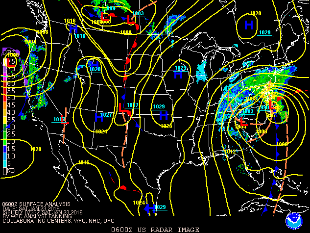
Regional snowfall amounts:
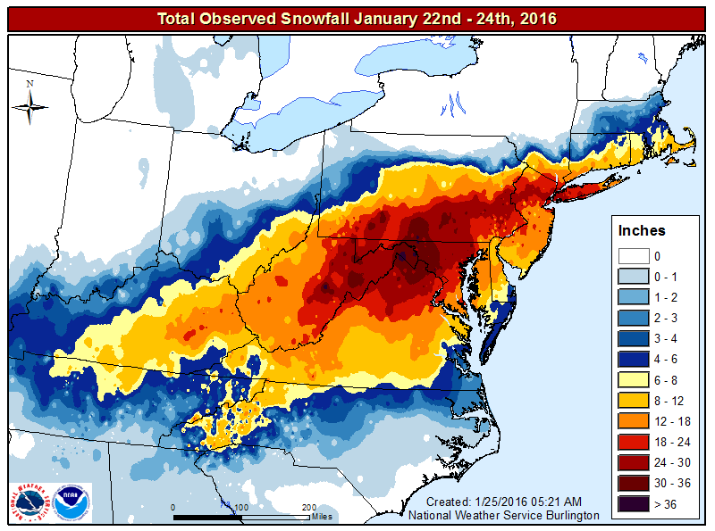
Set up environment
Set up environmentSet Up Environment
To run the snow storm case, first set up the environment for this case study.
| tcsh | bash |
|---|---|
|
cd /home/ec2-user
setenv PROJ_DIR `pwd` setenv PROJ_VERSION 4.1.0
|
cd /home/ec2-user
export PROJ_DIR=`pwd` export PROJ_VERSION="4.1.0"
|
Then, you should set up the variables and directories for the snow storm case:
| For tcsh: | For bash: |
|---|---|
|
setenv CASE_DIR ${PROJ_DIR}/snow
|
export CASE_DIR=${PROJ_DIR}/snow
|
cd ${CASE_DIR}
mkdir -p wpsprd wrfprd gsiprd postprd pythonprd metprd metviewer/mysql
Extra step for singularity users
Users of singularity containerization software will need to set a special variable for temporary files written by singularity at runtime:
| tcsh | bash |
|---|---|
|
setenv TMPDIR ${PROJ_DIR}/snow/tmp
|
export TMPDIR=${PROJ_DIR}/snow/tmp
|
Run NWP initialization components
Run NWP initialization componentsRun NWP Initialization Components
The NWP workflow process begins by creating the initial and boundary conditions for running the WRF model. This will be done in two steps using WPS (geogrid.exe, ungrib.exe, metgrid.exe) and WRF (real.exe) programs.
Initialization Data
Global Forecast System (GFS) forecast files initialized at 00 UTC on 20160123 out 24 hours in 3-hr increments are provided for this case.
Model Domain
The WRF domain we have selected covers the contiguous United States. The exact domain is shown below:
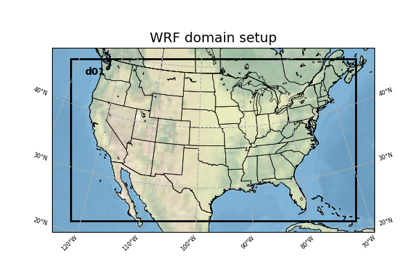
SELECT THE APPROPRIATE CONTAINER INSTRUCTIONS FOR YOUR SYSTEM BELOW:
Step One (Optional): Run Python to Create Image of Domain
A Python script has been provided to plot the computational domain that is being run for this case. If desired, run the dtcenter/python container to execute Python in docker-space using the namelist.wps in the local scripts directory, mapping the output into the local pythonprd directory.
-v ${PROJ_DIR}/container-dtc-nwp/components/scripts/common:/home/scripts/common \
-v ${PROJ_DIR}/container-dtc-nwp/components/scripts/snow_20160123:/home/scripts/case \
-v ${PROJ_DIR}/data/shapefiles:/home/data/shapefiles \
-v ${CASE_DIR}/pythonprd:/home/pythonprd \
--name run-snow-python dtcenter/python:${PROJ_VERSION} \
/home/scripts/common/run_python_domain.ksh
A successful completion of the Python plotting script will result in the following file in the pythonprd directory. This is the same image that is shown at the top of the page showing the model domain.
Step Two: Run WPS
Using the previously downloaded data (in ${PROJ_DIR}/data), while pointing to the namelists in the local scripts directory, run the dtcenter/wps_wrf container to run WPS in docker-space and map the output into the local wpsprd directory.
-v ${PROJ_DIR}/data/WPS_GEOG:/data/WPS_GEOG -v ${PROJ_DIR}/data:/data \
-v ${PROJ_DIR}/container-dtc-nwp/components/scripts/common:/home/scripts/common \
-v ${CASE_DIR}/wrfprd:/home/wrfprd -v ${CASE_DIR}/wpsprd:/home/wpsprd \
-v ${PROJ_DIR}/container-dtc-nwp/components/scripts/snow_20160123:/home/scripts/case \
--name run-dtc-nwp-snow dtcenter/wps_wrf:${PROJ_VERSION} /home/scripts/common/run_wps.ksh
Once WPS begins running, you can watch the log files being generated in another window by setting the ${CASE_DIR} environment variable and tailing the log files:
Type CTRL-C to exit the tail utility.
A successful completion of the WPS steps will result in the following files (in addition to other files) in the wpsprd directory
FILE:2016-01-23_00
FILE:2016-01-23_03
FILE:2016-01-23_06
FILE:2016-01-23_09
FILE:2016-01-23_12
FILE:2016-01-23_15
FILE:2016-01-23_18
FILE:2016-01-23_21
FILE:2016-01-24_00
met_em.d01.2016-01-23_00:00:00.nc
met_em.d01.2016-01-23_03:00:00.nc
met_em.d01.2016-01-23_06:00:00.nc
met_em.d01.2016-01-23_09:00:00.nc
met_em.d01.2016-01-23_12:00:00.nc
met_em.d01.2016-01-23_15:00:00.nc
met_em.d01.2016-01-23_18:00:00.nc
met_em.d01.2016-01-23_21:00:00.nc
met_em.d01.2016-01-24_00:00:00.nc
Step Three: Run real.exe
Using the previously downloaded data (in ${PROJ_DIR}/data), output from WPS in step one, and pointing to the namelists in the local scripts directory, run the dtcenter/wps_wrf container to this time run real.exe in docker-space and map the output into the local wrfprd directory.
-v ${PROJ_DIR}/data:/data -v ${PROJ_DIR}/container-dtc-nwp/components/scripts/common:/home/scripts/common \
-v ${CASE_DIR}/wrfprd:/home/wrfprd -v ${CASE_DIR}/wpsprd:/home/wpsprd \
-v ${PROJ_DIR}/container-dtc-nwp/components/scripts/snow_20160123:/home/scripts/case \
--name run-dtc-nwp-snow dtcenter/wps_wrf:${PROJ_VERSION} /home/scripts/common/run_real.ksh
The real.exe program should take less than a minute to run, but you can follow its progress as well in the wrfprd directory:
Type CTRL-C to exit the tail utility.
Step One (Optional): Run Python to Create Image of Domain
A Python script has been provided to plot the computational domain that is being run for this case. If desired, run the dtcenter/python container to execute Python in singularity-space using the namelist.wps in the local scripts directory, mapping the output into the local pythonprd directory.
A successful completion of the Python plotting script will result in the following file in the pythonprd directory. This is the same image that is shown at the top of the page showing the model domain.
Step Two: Run WPS
Using the previously downloaded data (in ${PROJ_DIR}/data), while pointing to the namelists in the local scripts directory, run the dtcenter/wps_wrf container to run WPS in singularity-space and map the output into the local wpsprd directory.
Once WPS begins running, you can watch the log files being generated in another window by setting the ${CASE_DIR} environment variable and tailing the log files:
Type CTRL-C to exit the tail utility.
Step Three: Run real.exe
Using the previously downloaded data (in ${PROJ_DIR}/data), output from WPS in step one, and pointing to the namelists in the local scripts directory, run the dtcenter/wps_wrf container to this time run real.exe in singularity-space and map the output into the local wrfprd directory.
The real.exe program should take less than a minute to run, but you can follow its progress as well in the wrfprd directory:
Type CTRL-C to exit the tail utility.
A successful completion of the WPS steps will result in the following files (in addition to other files) in the wpsprd directory
FILE:2016-01-23_00
FILE:2016-01-23_03
FILE:2016-01-23_06
FILE:2016-01-23_09
FILE:2016-01-23_12
FILE:2016-01-23_15
FILE:2016-01-23_18
FILE:2016-01-23_21
FILE:2016-01-24_00
met_em.d01.2016-01-23_00:00:00.nc
met_em.d01.2016-01-23_03:00:00.nc
met_em.d01.2016-01-23_06:00:00.nc
met_em.d01.2016-01-23_09:00:00.nc
met_em.d01.2016-01-23_12:00:00.nc
met_em.d01.2016-01-23_15:00:00.nc
met_em.d01.2016-01-23_18:00:00.nc
met_em.d01.2016-01-23_21:00:00.nc
met_em.d01.2016-01-24_00:00:00.nc
Run Data Assimilation
Run Data AssimilationRun Data Assimilation
Our next step in the NWP workflow will be to run GSI data assimilation to achieve better initial conditions in the WRF model run. GSI (gsi.exe) updates the wrfinput file created by real.exe.
SELECT THE APPROPRIATE CONTAINER INSTRUCTIONS FOR YOUR SYSTEM BELOW:
Using the previously downloaded data (in ${PROJ_DIR}/data), while pointing to the namelist in the local scripts directory, run the dtcenter/gsi container to run GSI in docker-space and map the output into the local gsiprd directory:
-v ${PROJ_DIR}/container-dtc-nwp/components/scripts/common:/home/scripts/common \
-v ${CASE_DIR}/wrfprd:/home/wrfprd -v ${CASE_DIR}/wpsprd:/home/wpsprd -v ${CASE_DIR}/gsiprd:/home/gsiprd \
-v ${PROJ_DIR}/container-dtc-nwp/components/scripts/snow_20160123:/home/scripts/case \
--name run-dtc-gsi-snow dtcenter/gsi:${PROJ_VERSION} /home/scripts/common/run_gsi.ksh
As GSI is run the output files will appear in the local gsiprd/. Please review the contents of that directory to interrogate the data.
Once GSI begins running, you can watch the log file being generated in another window by setting the ${CASE_DIR} environment variable and tailing the log file:
Type CTRL-C to exit the tail.
A successful completion of the GSI step will result in the following files (in addition to other files) in the gsiprd directory
berror_stats
diag_*
fit_*
fort*
gsiparm.anl
*info
list_run_directory
prepburf
satbias*
stdout*
wrf_inout
wrfanl.2016012300
Using the previously downloaded data (in ${PROJ_DIR}/data), while pointing to the namelist in the local scripts directory, create a container using the gsi image to run GSI in singularity-space and map the output into the local gsiprd directory:
As GSI is run the output files will appear in the local gsiprd/. Please review the contents of that directory to interrogate the data.
Once GSI begins running, you can watch the log file being generated in another window by setting the ${CASE_DIR} environment variable and tailing the log file:
A successful completion of the GSI step will result in the following files (in addition to other files) in the gsiprd directory
berror_stats
diag_*
fit_*
fort*
gsiparm.anl
*info
list_run_directory
prepburf
satbias*
stdout*
wrf_inout
wrfanl.2016012300
Type CTRL-C to exit the tail.
Run NWP model
Run NWP modelRun NWP Model
To integrate the WRF forecast model through time, we use the wrf.exe program and point to the initial and boundary condition files created in the previous initialization, and optional data assimilation, step(s).
SELECT THE APPROPRIATE CONTAINER INSTRUCTIONS FOR YOUR SYSTEM BELOW:
Using the previously downloaded data (in ${PROJ_DIR}/data), while pointing to the namelists in the local scripts directory, run the dtcenter/wps_wrf container to run WRF in docker-space and map the output into the local wrfprd directory.
Note: Read the following two options carefully and decide which one is right for you to run - you DO NOT need to run both. Option One runs with 4 processors by default and Option Two allows for a user specified number of processors using the "-np #" option.
Option One: Default number (4) of processors
By default WRF will run with 4 processors using the following command:
-v ${PROJ_DIR}/container-dtc-nwp/components/scripts/common:/home/scripts/common \
-v ${CASE_DIR}/wrfprd:/home/wrfprd -v ${CASE_DIR}/wpsprd:/home/wpsprd \
-v ${PROJ_DIR}/container-dtc-nwp/components/scripts/snow_20160123:/home/scripts/case \
--name run-dtc-nwp-snow dtcenter/wps_wrf:${PROJ_VERSION} /home/scripts/common/run_wrf.ksh
Option Two: User-specified number of processors
If you run into trouble on your machine when using 4 processors, you may want to run with fewer (or more!) processors by passing the "-np #" option to the script. For example the following command runs with 2 processors:
-v ${PROJ_DIR}/container-dtc-nwp/components/scripts/common:/home/scripts/common \
-v ${CASE_DIR}/wrfprd:/home/wrfprd -v ${CASE_DIR}/wpsprd:/home/wpsprd \
-v ${PROJ_DIR}/container-dtc-nwp/components/scripts/snow_20160123:/home/scripts/case \
--name run-dtc-nwp-snow dtcenter/wps_wrf:${PROJ_VERSION} /home/scripts/common/run_wrf.ksh -np 2
As WRF is run the NetCDF output files will appear in the local wrfprd/. Please review the contents of that directory to interrogate the data.
Once WRF begins running, you can watch the log file being generated in another window by setting the ${CASE_DIR} environment variable and tailing the log file:
Type CTRL-C to exit the tail.
A successful completion of the WRF step will result in the following files (in addition to other files) in the wrfprd directory:
wrfout_d01_2016-01-23_01_00_00.nc
wrfout_d01_2016-01-23_02_00_00.nc
wrfout_d01_2016-01-23_03_00_00.nc
...
wrfout_d01_2016-01-23_22_00_00.nc
wrfout_d01_2016-01-23_23_00_00.nc
wrfout_d01_2016-01-24_00_00_00.nc
Using the previously downloaded data in ${PROJ_DIR}/data, while pointing to the namelists in the local scripts directory, create a container from the wps_wrf image to run WRF in singularity-space and map the output into the local wrfprd directory.
Note: Read the following two options carefully and decide which one is right for you to run - you DO NOT need to run both. Option One runs with 4 processors by default and Option Two allows for a user specified number of processors using the "-np #" option.
Option One: Default number (4) of processors
By default WRF will run with 4 processors using the following command:
Option Two: User-specified number of processors
If you run into trouble on your machine when using 4 processors, you may want to run with fewer (or more!) processors by passing the "-np #" option to the script. For example the following command runs with 2 processors:
As WRF is run the NetCDF output files will appear in the local wrfprd/. Please review the contents of that directory to interrogate the data.
Once WRF begins running, you can watch the log file being generated in another window by setting the ${CASE_DIR} environment variable and tailing the log file:
tail -f ${CASE_DIR}/wrfprd/rsl.out.0000
Type CTRL-C to exit the tail.
A successful completion of the WRF step will result in the following files (in addition to other files) in the wrfprd directory:
wrfout_d01_2016-01-23_01_00_00.nc
wrfout_d01_2016-01-23_02_00_00.nc
wrfout_d01_2016-01-23_03_00_00.nc
...
wrfout_d01_2016-01-23_22_00_00.nc
wrfout_d01_2016-01-23_23_00_00.nc
wrfout_d01_2016-01-24_00_00_00.nc
Postprocess NWP data
Postprocess NWP dataPostprocess NWP Data
After the WRF model is run, the output is run through the Unified Post Processor (UPP) to interpolate model output to new vertical coordinates, e.g. pressure levels, and compute a number diagnostic variables that are output in GRIB2 format.
SELECT THE APPROPRIATE CONTAINER INSTRUCTIONS FOR YOUR SYSTEM BELOW:
Using the previously created netCDF wrfout files in the wrfprd directory, while pointing to the namelist in the local scripts directory, run the dtcenter/upp container to run UPP in docker-space to post-process the WRF data into grib2 format, and map the output into the local postprd directory:
docker run --rm -it -e LOCAL_USER_ID=`id -u $USER` \
-v ${PROJ_DIR}/container-dtc-nwp/components/scripts/common:/home/scripts/common \
-v ${PROJ_DIR}/container-dtc-nwp/components/scripts/snow_20160123:/home/scripts/case \
-v ${CASE_DIR}/wrfprd:/home/wrfprd -v ${CASE_DIR}/postprd:/home/postprd \
--name run-snow-upp dtcenter/upp:${PROJ_VERSION} /home/scripts/common/run_upp.ksh
As UPP is run, the post-processed GRIB output files will appear in the postprd/. Please review the contents of that directory to interrogate the data.
UPP runs quickly for each forecast hour, but you can see the log files generated in another window by setting the ${CASE_DIR} environment variable and tailing the log files:
Type CTRL-C to exit the tail.
A successful completion of the UPP step will result in the following files (in addition to other files) in the postprd directory:
wrfprs_d01.01
wrfprs_d01.02
wrfprs_d01.03
...
wrfprs_d01.23
wrfprs_d01.24
Using the previously created netCDF wrfout data in the wrfprd directory, while pointing to the namelists in the local scripts directory, create a container using the upp image to run UPP in singularity-space and map the output into the local postprd directory:
As UPP is run the post-processed GRIB output files will appear in the postprd/. Please review the contents of those directories to interrogate the data.
UPP runs quickly for each forecast hour, but you can see the log files generated in another window by setting the ${CASE_DIR} environment variable and tailing the log file:
Type CTRL-C to exit the tail.
A successful completion of the UPP step will result in the following files (in addition to other files) in the postprd directory:
wrfprs_d01.01
wrfprs_d01.02
wrfprs_d01.03
...
wrfprs_d01.23
wrfprs_d01.24
Create graphics
Create graphicsCreate Graphics
After the model output is post-processed with UPP, the forecast fields can be visualized using Python. The plotting capabilities include generating graphics for near-surface and upper-air variables as well as accumulated precipitation, reflectivity, helicity, and CAPE.
SELECT THE APPROPRIATE CONTAINER INSTRUCTIONS FOR YOUR SYSTEM BELOW:
Pointing to the scripts in the local scripts directory, run the dtcenter/python container to create graphics in docker-space and map the images into the local pythonprd directory:
-v ${PROJ_DIR}/container-dtc-nwp/components/scripts/common:/home/scripts/common \
-v ${PROJ_DIR}/container-dtc-nwp/components/scripts/snow_20160123:/home/scripts/case \
-v ${PROJ_DIR}/data/shapefiles:/home/data/shapefiles \
-v ${CASE_DIR}/postprd:/home/postprd -v ${CASE_DIR}/pythonprd:/home/pythonprd \
--name run-snow-python dtcenter/python:${PROJ_VERSION} /home/scripts/common/run_python.ksh
After Python has been run, the plain image output files will appear in the local pythonprd/ directory.
250wind_d01_f*.png
2mdew_d01_f*.png
2mt_d01_f*.png
500_d01_f*.png
maxuh25_d01_f*.png
qpf_d01_f*.png
refc_d01_f*.png
sfcape_d01_f*.png
slp_d01_f*.png
The images may be visualized using your favorite display tool.
Pointing to the scripts in the local scripts directory, create a container using the python_3.5 singularity image to create graphics in singularity-space and map the images into the local pythonprd directory:
After Python has been run, the plain image output files will appear in the local pythonprd/ directory.
250wind_d01_f*.png
2mdew_d01_f*.png
2mt_d01_f*.png
500_d01_f*.png
maxuh25_d01_f*.png
qpf_d01_f*.png
refc_d01_f*.png
sfcape_d01_f*.png
slp_d01_f*.png
The images may be visualized using your favorite display tool.
Run verification software
Run verification softwareRun Verification Software
After the model output is post-processed with UPP, it is run through the Model Evaluation Tools (MET) software to quantify its performance relative to observations. State variables, including temperature, dewpoint, and wind, are verified against both surface and upper-air point observations, while precipitation is verified against a gridded analysis.
SELECT THE APPROPRIATE CONTAINER INSTRUCTIONS FOR YOUR SYSTEM BELOW:
Using the previously downloaded data (in ${PROJ_DIR}/data), while pointing to the output in the local scripts and postprd directories, run the dtcenter/met container to run the verification software in docker-space and map the statistical output into the local metprd directory:
-v ${PROJ_DIR}/data:/data \
-v ${PROJ_DIR}/container-dtc-nwp/components/scripts/common:/home/scripts/common \
-v ${PROJ_DIR}/container-dtc-nwp/components/scripts/snow_20160123:/home/scripts/case \
-v ${CASE_DIR}/postprd:/home/postprd -v ${CASE_DIR}/metprd:/home/metprd \
--name run-snow-met dtcenter/nwp-container-met:${PROJ_VERSION} /home/scripts/common/run_met.ksh
MET will write a variety of ASCII and netCDF output files to the local metprd/. Please review the contents of the directories: grid_stat, pb2nc, pcp_combine, and point_stat, to interrogate the data.
grid_stat/grid_stat*.stat
pb2nc/prepbufr*.nc
pcp_combine/ST2*.nc
pcp_combine/wrfprs*.nc
point_stat/point_stat*.stat
Using the previously downloaded data (in ${PROJ_DIR}/data), while pointing to the output in the local scripts and postprd directories, create a container using the nwp-container-met image to run the verification software in singularity-space and map the statistical output into the local metprd directory:
MET will write a variety of ASCII and netCDF output files to the local metprd/. Please review the contents of the directories: grid_stat, pb2nc, pcp_combine, and point_stat, to interrogate the data.
grid_stat/grid_stat*.stat
pb2nc/prepbufr*.nc
pcp_combine/ST2*.nc
pcp_combine/wrfprs*.nc
point_stat/point_stat*.stat
Visualize verification results
Visualize verification resultsVisualize Verification Results
The METviewer software provides a database and display system for visualizing the statistical output generated by MET. After starting the METviewer service, a new database is created into which the MET output is loaded. Plots of the verification statistics are created by interacting with a web-based graphical interface.
SELECT THE APPROPRIATE CONTAINER INSTRUCTIONS FOR YOUR SYSTEM BELOW:
In order to visualize the MET output using the METviewer database and display system, you first need to launch the METviewer container.
docker-compose up -d
The MET statistical output then needs to be loaded into the MySQL database for querying and plotting by METviewer
The METviewer GUI can then be accessed with the following URL copied and pasted into your web browser:
Note, if you are running on AWS, run the following commands to reconfigure METviewer with your current IP address and restart the web service:
|
docker exec -it metviewer /bin/bash
/scripts/common/reset_metv_url.ksh exit |
The METviewer GUI can then be accessed with the following URL copied and pasted into your web browser (where IPV4_public_IP is your IPV4Public IP from the AWS “Active Instances” web page):
http://IPV4_public_IP:8080/metviewer/metviewer1.jsp
The METviewer GUI can be run interactively to create verification plots on the fly. However, to get you going, two sample plots are provided. Do the following in the METviewer GUI:
-
Click the "Choose File" button and navigate on your file system to:
${PROJ_DIR}/container-dtc-nwp/components/scripts/snow_20160123/metviewer/plot_APCP_03_ETS.xml
-
Click "OK" to load the XML to the GUI and populate all the required options.
-
Click the "Generate Plot" button on the top of the page to create the image.
Next, follow the same steps to create a plot of 10-meter wind components with this XML file:
Feel free to make changes in the METviewer GUI and use the "Generate Plot" button to make new plots. For example, the following plot was created by changing the "Independent Variable" field to "VALID_HOUR", including times from 0 through 12 hours, and changing the X label appropriately:
Note: Use of METviewer with Singularity is only supported on AWS!
In order to visualize the MET output using the METviewer database and display system, you first need to build Singularity sandbox from the docker container using 'fix-perms' options. The execution of this step creates a metv4singularity directory.
singularity build --sandbox --fix-perms --force metv4singularity docker://dtcenter/nwp-container-metviewer-for-singularity:${PROJ_VERSION}
Next, start the Singularity instance as 'writable' and call it 'metv':
Then, initialize and start MariaDB and Tomcat:
Then, navigate to the scripts area and run a shell in the Singularity container:
singularity shell instance://metv
Now it is time to load the MET output into a METviewer database. As a note, the metv_load_singularity.ksh script requires two command-line arguments: 1) name of the METviewer database (e.g., mv_snow), and 2) the ${CASE_DIR}
The METviewer GUI can then be accessed with the following URL copied and pasted into your web browser (where IPV4_public_IP is your IPV4Public IP from the AWS “Active Instances” web page):
http://IPV4_public_IP:8080/metviewer/metviewer1.jsp
Click the "Load XML" button in the top-right corner.
The METviewer GUI can be run interactively to create verification plots on the fly. However, to get you going, two sample plots are provided. Do the following in the METviewer GUI:
-
Click the "Choose File" button and navigate on your file system to:
${PROJ_DIR}/container-dtc-nwp/components/scripts/snow_20160123/metviewer/plot_APCP_03_ETS.xml
-
Click "OK" to load the XML to the GUI and populate all the required options.
-
Click the "Generate Plot" button on the top of the page to create the image.
Next, follow the same steps to create a plot of 10-meter wind components with this XML file:
Feel free to make changes in the METviewer GUI and use the "Generate Plot" button to make new plots.
You can also create plots via the METviewer batch plotting capability (i.e., not the METviewer GUI). A script to run the two supplied METviewer XMLs provides an example on how to create plots. Note you must be in your metviewer singularity shell to run it, as shown below:
singularity shell instance://metv
cd ${PROJ_DIR}/container-dtc-nwp/components/scripts/snow_20160123/metviewer ./metv_plot_singularity.ksh ${CASE_DIR}
The output goes to: ${CASE_DIR}/metviewer/plots, and you can use display to view the images.
Derecho Case (29 Jun 2012)
Derecho Case (29 Jun 2012)Case overview
Reason for interest: Very strong, high-impact derecho
A deadly, record-setting derecho on this day was preceded by major instability from the Midwest to the East Coast of the United States, with CAPE values exceeding 5000 J/kg and temperatures reaching above 100°F (38°C). Elevated convection in northern Illinois moved into Indiana along a weak stationary front, above an elevated mixed layer. Record temperatures, abundant moisture, and steep lapse rates aided further storm development to the south and east. A squall line eventually formed into a bow echo and wreaked havoc from Illinois over the Appalachian Mountains all the way to the Atlantic coast.
More than 20 fatalities resulted from high winds and falling trees, and over 4 million people lost power. There were 893 high wind reports for June 29th, 2012, with some reaching over 90 mph.
SPC Storm Reports for June 29th, 2012:
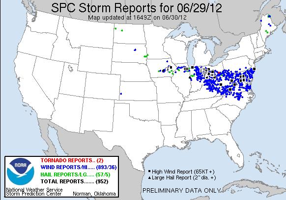
Storm Summary from NWS/SPC:
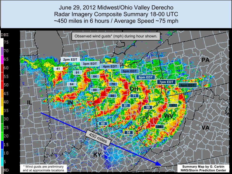
Set up environment
Set up environmentSet Up Environment
| tcsh | bash |
|---|---|
|
cd /home/ec2-user
setenv PROJ_DIR `pwd` setenv PROJ_VERSION 4.1.0
|
cd /home/ec2-user
export PROJ_DIR=`pwd` export PROJ_VERSION="4.1.0"
|
| For tcsh: | For bash: |
|---|---|
|
setenv CASE_DIR ${PROJ_DIR}/derecho
|
export CASE_DIR=${PROJ_DIR}/derecho
|
cd ${CASE_DIR}
mkdir -p wpsprd wrfprd gsiprd postprd pythonprd metprd metviewer/mysql
Extra step for singularity users
Users of singularity containerization software will need to set a special variable for temporary files written by singularity at runtime:
| tcsh | bash |
|---|---|
|
setenv TMPDIR ${PROJ_DIR}/derecho/tmp
|
export TMPDIR=${PROJ_DIR}/derecho/tmp
|
Run NWP initialization components
Run NWP initialization componentsRun NWP Initialization Components
The NWP workflow process begins by creating the initial and boundary conditions for running the WRF model. This will be done in two steps using WPS (geogrid.exe, ungrib.exe, metgrid.exe) and WRF (real.exe) programs.
Initialization Data
Global Forecast System (GFS) forecast files initialized at 12 UTC on 20120629 out 24 hours in 3-hr increments are provided for this case.
Model Domain
This case uses the nesting functionality of WRF: instead of one domain at a single resolution, this WRF run has one larger, coarser-resolution domain, and a smaller, finer-resolution domain within it. The outer WRF domain we have selected for this case covers the Ohio River region in the eastern United States, while the nested domain covers a portion of southern Ohio and far-northeastern Kentucky. The exact domains are shown below:
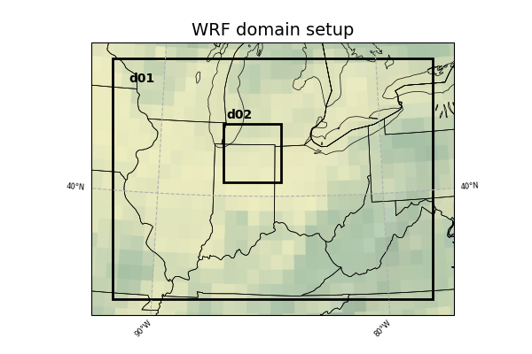
SELECT THE APPROPRIATE CONTAINER INSTRUCTIONS FOR YOUR SYSTEM BELOW:
Step One (Optional): Run Python to Create Image of Domain
A Python script has been provided to plot the computational domain that is being run for this case. If desired, run the dtcenter/python container to execute Python in docker-space using the namelist.wps in the local scripts directory, mapping the output into the local pythonprd directory.
-v ${PROJ_DIR}/container-dtc-nwp/components/scripts/common:/home/scripts/common \
-v ${PROJ_DIR}/container-dtc-nwp/components/scripts/derecho_20120629:/home/scripts/case \
-v ${PROJ_DIR}/data/shapefiles:/home/data/shapefiles \
-v ${CASE_DIR}/pythonprd:/home/pythonprd \
--name run-derecho-python dtcenter/python:${PROJ_VERSION} \
/home/scripts/common/run_python_domain.ksh
A successful completion of the Python plotting script will result in the following file in the pythonprd directory. This is the same image that is shown at the top of the page showing the model domain.
Step Two: Run WPS
Using the previously downloaded data (in ${PROJ_DIR}/data), while pointing to the namelists in the local scripts directory, run the dtcenter/wps_wrf container to run WPS in docker-space and map the output into the local wpsprd directory.
-v ${PROJ_DIR}/data/WPS_GEOG:/data/WPS_GEOG -v ${PROJ_DIR}/data:/data \
-v ${PROJ_DIR}/container-dtc-nwp/components/scripts/common:/home/scripts/common \
-v ${CASE_DIR}/wrfprd:/home/wrfprd -v ${CASE_DIR}/wpsprd:/home/wpsprd \
-v ${PROJ_DIR}/container-dtc-nwp/components/scripts/derecho_20120629:/home/scripts/case \
--name run-dtc-nwp-derecho dtcenter/wps_wrf:${PROJ_VERSION} /home/scripts/common/run_wps.ksh
Once WPS begins running, you can watch the log files being generated in another window by setting the ${CASE_DIR} environment variable and tailing the log files:
Type CTRL-C to exit the tail utility.
A successful completion of the WPS steps will result in the following files (in addition to other files) in the wpsprd directory
geo_em.d02.nc
FILE:2012-06-29_12
FILE:2012-06-29_15
FILE:2012-06-29_18
...
FILE:2012-06-30_09
FILE:2012-06-30_12
met_em.d01.2012-06-29_12:00:00.nc
met_em.d01.2012-06-29_15:00:00.nc
met_em.d01.2012-06-29_18:00:00.nc
...
met_em.d01.2012-06-30_09:00:00.nc
met_em.d01.2012-06-30_12:00:00.nc
met_em.d02.2012-06-30_03:00:00.nc
met_em.d02.2012-06-30_06:00:00.nc
met_em.d02.2012-06-30_09:00:00.nc
Step Three: Run real.exe
Using the previously downloaded data (in ${PROJ_DIR}/data), output from WPS in step one, and pointing to the namelists in the local scripts directory, run the dtcenter/wps_wrf container to this time run real.exe in docker-space and map the output into the local wrfprd directory.
-v ${PROJ_DIR}/data:/data -v ${PROJ_DIR}/container-dtc-nwp/components/scripts/common:/home/scripts/common \
-v ${CASE_DIR}/wrfprd:/home/wrfprd -v ${CASE_DIR}/wpsprd:/home/wpsprd \
-v ${PROJ_DIR}/container-dtc-nwp/components/scripts/derecho_20120629:/home/scripts/case \
--name run-dtc-nwp-derecho dtcenter/wps_wrf:${PROJ_VERSION} /home/scripts/common/run_real.ksh
The real.exe program should take less than a minute to run, but you can follow its progress as well in the wrfprd directory:
Type CTRL-C to exit the tail utility.
A successful completion of the REAL step will result in the following files (in addition to other files) in the wrfprd directory
wrfinput_d01
wrfinput_d02
Step One (Optional): Run Python to Create Image of Domain
A Python script has been provided to plot the computational domain that is being run for this case. If desired, run the dtcenter/python container to execute Python in singularity-space using the namelist.wps in the local scripts directory, mapping the output into the local pythonprd directory.
A successful completion of the Python plotting script will result in the following file in the pythonprd directory. This is the same image that is shown at the top of the page showing the model domain.
Step Two: Run WPS
Using the previously downloaded data (in ${PROJ_DIR}/data), while pointing to the namelists in the local scripts directory, run the wps_wrf container to run WPS in singularity-space and map the output into the local wpsprd directory.
Once WPS begins running, you can watch the log files being generated in another window by setting the ${CASE_DIR} environment variable and tailing the log files:
Type CTRL-C to exit the tail utility.
A successful completion of the WPS steps will result in the following files (in addition to other files) in the wpsprd directory
geo_em.d02.nc
FILE:2012-06-29_12
FILE:2012-06-29_15
FILE:2012-06-29_18
...
FILE:2012-06-30_09
FILE:2012-06-30_12
met_em.d01.2012-06-29_12:00:00.nc
met_em.d01.2012-06-29_15:00:00.nc
met_em.d01.2012-06-29_18:00:00.nc
...
met_em.d01.2012-06-30_09:00:00.nc
met_em.d01.2012-06-30_12:00:00.nc
met_em.d02.2012-06-30_03:00:00.nc
met_em.d02.2012-06-30_06:00:00.nc
met_em.d02.2012-06-30_09:00:00.nc
Step Three: Run real.exe
Using the previously downloaded data (in ${PROJ_DIR}/data), output from WPS in step one, and pointing to the namelists in the local scripts directory, run the dtcenter/wps_wrf container to this time run real.exe in singularity-space and map the output into the local wrfprd directory.
The real.exe program should take less than a minute to run, but you can follow its progress as well in the wrfprd directory:
Type CTRL-C to exit the tail utility.
A successful completion of the REAL step will result in the following files (in addition to other files) in the wrfprd directory
wrfinput_d01
wrfinput_d02
Run data assimilation
Run data assimilationRun Data Assimilation
Our next step in the NWP workflow will be to run GSI data assimilation to achieve better initial conditions in the WRF model run. GSI (gsi.exe) updates the wrfinput file created by real.exe.
SELECT THE APPROPRIATE CONTAINER INSTRUCTIONS FOR YOUR SYSTEM BELOW:
Using the previously downloaded data (in ${PROJ_DIR}/data), while pointing to the namelist in the local scripts directory, run the dtcenter/gsi container to run GSI in docker-space and map the output into the local gsiprd directory:
-v ${PROJ_DIR}/data:/data \
-v ${PROJ_DIR}/container-dtc-nwp/components/scripts/common:/home/scripts/common \
-v ${CASE_DIR}/wrfprd:/home/wrfprd -v ${CASE_DIR}/wpsprd:/home/wpsprd -v ${CASE_DIR}/gsiprd:/home/gsiprd \
-v ${PROJ_DIR}/container-dtc-nwp/components/scripts/derecho_20120629:/home/scripts/case \
--name run-dtc-gsi-derecho dtcenter/gsi:${PROJ_VERSION} /home/scripts/common/run_gsi.ksh
As GSI is run the output files will appear in the local gsiprd/. Please review the contents of that directory to interrogate the data.
Once GSI begins running, you can watch the log file being generated in another window by setting the ${CASE_DIR} environment variable and tailing the log file:
Type CTRL-C to exit the tail.
A successful completion of the GSI step will result in the following files (in addition to other files) in the gsiprd directory
berror_stats
diag_*
fit_*
fort*
gsiparm.anl
*info
list_run_directory
prepburf
satbias*
stdout*
wrf_inout
wrfanl.2012062912
Using the previously downloaded data (in ${PROJ_DIR}/data), while pointing to the namelist in the local scripts directory, create a container using the gsi image to run GSI in singularity-space and map the output into the local gsiprd directory:
As GSI is run the output files will appear in the local gsiprd/. Please review the contents of that directory to interrogate the data.
Once GSI begins running, you can watch the log file being generated in another window by setting the ${CASE_DIR} environment variable and tailing the log file:
Type CTRL-C to exit the tail.
A successful completion of the GSI step will result in the following files (in addition to other files) in the gsiprd directory
berror_stats
diag_*
fit_*
fort*
gsiparm.anl
*info
list_run_directory
prepburf
satbias*
stdout*
wrf_inout
wrfanl.2012062912
Run NWP model
Run NWP modelRun NWP Model
To integrate the WRF forecast model through time, we use the wrf.exe program and point to the initial and boundary condition files created in the previous initialization, and optional data assimilation, step(s).
SELECT THE APPROPRIATE CONTAINER INSTRUCTIONS FOR YOUR SYSTEM BELOW:
Using the previously downloaded data (in ${PROJ_DIR}/data), while pointing to the namelists in the local scripts directory, run the dtcenter/wps_wrf container to run WRF in docker-space and map the output into the local wrfprd directory.
Note: Read the following two options carefully and decide which one is right for you to run - you DO NOT need to run both. Option One runs with 4 processors by default and Option Two allows for a user specified number of processors using the "-np #" option.
Option One: Default number (4) of processors
By default WRF will run with 4 processors using the following command:
-v ${PROJ_DIR}/container-dtc-nwp/components/scripts/common:/home/scripts/common \
-v ${CASE_DIR}/wrfprd:/home/wrfprd -v ${CASE_DIR}/wpsprd:/home/wpsprd \
-v ${PROJ_DIR}/container-dtc-nwp/components/scripts/derecho_20120629:/home/scripts/case \
--name run-dtc-nwp-derecho dtcenter/wps_wrf:${PROJ_VERSION} /home/scripts/common/run_wrf.ksh
Option Two: User-specified number of processors
If you run into trouble on your machine when using 4 processors, you may want to run with fewer (or more!) processors by passing the "-np #" option to the script. For example the following command runs with 2 processors:
-v ${PROJ_DIR}/container-dtc-nwp/components/scripts/common:/home/scripts/common \
-v ${CASE_DIR}/wrfprd:/home/wrfprd -v ${CASE_DIR}/wpsprd:/home/wpsprd \
-v ${PROJ_DIR}/container-dtc-nwp/components/scripts/derecho_20120629:/home/scripts/case \
--name run-dtc-nwp-derecho dtcenter/wps_wrf:${PROJ_VERSION} /home/scripts/common/run_wrf.ksh -np 2
As WRF is run the NetCDF output files will appear in the local wrfprd/. Please review the contents of that directory to interrogate the data.
Once WRF begins running, you can watch the log file being generated in another window by setting the ${CASE_DIR} environment variable and tailing the log file:
Type CTRL-C to exit the tail.
A successful completion of the WRF step will result in the following files (in addition to other files) in the wrfprd directory:
wrfout_d01_2012-06-29_15_00_00.nc
wrfout_d01_2012-06-29_18_00_00.nc
...
wrfout_d01_2012-06-30_09_00_00.nc
wrfout_d01_2012-06-30_12_00_00.nc
wrfout_d02_2012-06-30_03_00_00.nc
wrfout_d02_2012-06-30_06_00_00.nc
wrfout_d02_2012-06-30_09_00_00.nc
Using the previously downloaded data in ${PROJ_DIR}/data while pointing to the namelists in the local scripts directory, run the wps_wrf container to run WRF in singularity-space and map the output into the local wrfprd directory.
Note: Read the following two options carefully and decide which one is right for you to run - you DO NOT need to run both. Option One runs with 4 processors by default and Option Two allows for a user specified number of processors using the "-np #" option.
Option One: Default number (4) of processors
By default WRF will run with 4 processors using the following command:
Option Two: User-specified number of processors
If you run into trouble on your machine when using 4 processors, you may want to run with fewer (or more!) processors by passing the "-np #" option to the script. For example the following command runs with 2 processors:
As WRF is run the NetCDF output files will appear in the local wrfprd/. Please review the contents of that directory to interrogate the data.
Once WRF begins running, you can watch the log file being generated in another window by setting the ${CASE_DIR} environment variable and tailing the log file:
A successful completion of the WRF step will result in the following files (in addition to other files) in the wrfprd directory:
wrfout_d01_2012-06-29_15_00_00.nc
wrfout_d01_2012-06-29_18_00_00.nc
...
wrfout_d01_2012-06-30_09_00_00.nc
wrfout_d01_2012-06-30_12_00_00.nc
wrfout_d02_2012-06-30_03_00_00.nc
wrfout_d02_2012-06-30_06_00_00.nc
wrfout_d02_2012-06-30_09_00_00.nc
Type CTRL-C to exit the tail.
Postprocess NWP data
Postprocess NWP dataPostprocess NWP Data
After the WRF model is run, the output is run through the Unified Post Processor (UPP) to interpolate model output to new vertical coordinates, e.g. pressure levels, and compute a number diagnostic variables that are output in GRIB2 format.
SELECT THE APPROPRIATE CONTAINER INSTRUCTIONS FOR YOUR SYSTEM BELOW:
Using the previously created WRF netCDF data in the wrfprd directory, while pointing to the namelist in the local scripts directory, run the dtcenter/upp container to run UPP in docker-space to post-process the WRF data into grib2 format, and map the output into the local postprd directory:
-v ${PROJ_DIR}/container-dtc-nwp/components/scripts/common:/home/scripts/common \
-v ${PROJ_DIR}/container-dtc-nwp/components/scripts/derecho_20120629:/home/scripts/case \
-v ${CASE_DIR}/wrfprd:/home/wrfprd -v ${CASE_DIR}/postprd:/home/postprd \
--name run-derecho-upp dtcenter/upp:${PROJ_VERSION} /home/scripts/common/run_upp.ksh
As UPP is run the post-processed GRIB output files will appear in the postprd/. Please review the contents of those directories to interrogate the data.
UPP runs quickly for each forecast hour, but you can see the log files generated in another window by setting the ${CASE_DIR} environment variable and tailing the log file:
Type CTRL-C to exit the tail.
A successful completion of the UPP step will result in the following files (in addition to other files) in the postprd directory:
wrfprs_d01.03
wrfprs_d01.06
...
wrfprs_d01.21
wrfprs_d01.24
wrfprs_d02.15
wrfprs_d02.18
wrfprs_d02.21
Using the previously created netCDF wrfout data in the wrfprd directory, while pointing to the namelists in the local scripts directory, create a container using the upp image to run WRF in singularity-space and map the output into the local postprd directory:
As UPP is run the post-processed GRIB output files will appear in the postprd/. Please review the contents of those directories to interrogate the data.
UPP runs quickly for each forecast hour, but you can see the log files generated in another window by setting the ${CASE_DIR} environment variable and tailing the log file:
A successful completion of the UPP step will result in the following files (in addition to other files) in the postprd directory:
wrfprs_d01.03
wrfprs_d01.06
...
wrfprs_d01.21
wrfprs_d01.24
wrfprs_d02.15
wrfprs_d02.18
wrfprs_d02.21
Type CTRL-C to exit the tail.
Create graphics
Create graphicsCreate Graphics
After the model output is post-processed with UPP, the forecast fields can be visualized using Python. The plotting capabilities include generating graphics for near-surface and upper-air variables as well as accumulated precipitation, reflectivity, helicity, and CAPE.
SELECT THE APPROPRIATE CONTAINER INSTRUCTIONS FOR YOUR SYSTEM BELOW:
Pointing to the scripts in the local scripts directory, run the dtcenter/python container to create graphics in docker-space and map the images into the local pythonprd directory:
-v ${PROJ_DIR}/container-dtc-nwp/components/scripts/common:/home/scripts/common \
-v ${PROJ_DIR}/container-dtc-nwp/components/scripts/derecho_20120629:/home/scripts/case \
-v ${PROJ_DIR}/data/shapefiles:/home/data/shapefiles \
-v ${CASE_DIR}/postprd:/home/postprd -v ${CASE_DIR}/pythonprd:/home/pythonprd \
--name run-derecho-python dtcenter/python:${PROJ_VERSION} /home/scripts/common/run_python.ksh
After Python has been run, the plain image output files will appear in the local pythonprd/ directory.
250wind_d0*.png
2mdew_d0*.png
2mt_d0*.png
500_d0*.png
maxuh25_d0*.png
qpf_d0*.png
refc_d0*.png
sfcape_d0*.png
slp_d0*.png
Pointing to the scripts in the local scripts directory, create a container using the python singularity image to create graphics in singularity-space and map the images into the local pythonprd directory:
After Python has been run, the plain image output files will appear in the local pythonprd/ directory.
250wind_d0*.png
2mdew_d0*.png
2mt_d0*.png
500_d0*.png
maxuh25_d0*.png
qpf_d0*.png
refc_d0*.png
sfcape_d0*.png
slp_d0*.png
Run verification software
Run verification softwareRun Verification Software
After the model output is post-processed with UPP, it is run through the Model Evaluation Tools (MET) software to quantify its performance relative to observations. State variables, including temperature, dewpoint, and wind, are verified against both surface and upper-air point observations, while precipitation is verified against a gridded analysis.
SELECT THE APPROPRIATE CONTAINER INSTRUCTIONS FOR YOUR SYSTEM BELOW:
Using the previously downloaded data (in ${PROJ_DIR}/data), while pointing to the output in the local scripts and postprd directories, run the dtcenter/nwp-container-met container to run the verification software in docker-space and map the statistical output into the local metprd directory:
-v ${PROJ_DIR}/data:/data \
-v ${PROJ_DIR}/container-dtc-nwp/components/scripts/common:/home/scripts/common \
-v ${PROJ_DIR}/container-dtc-nwp/components/scripts/derecho_20120629:/home/scripts/case \
-v ${CASE_DIR}/postprd:/home/postprd -v ${CASE_DIR}/metprd:/home/metprd \
--name run-derecho-met dtcenter/nwp-container-met:${PROJ_VERSION} /home/scripts/common/run_met.ksh
MET will write a variety of ASCII and netCDF output files to the local metprd/. Please review the contents of the directories: grid_stat, pb2nc, pcp_combine, and point_stat, to interrogate the data.
grid_stat/grid_stat*.stat
pb2nc/prepbufr*.nc
pcp_combine/ST2*.nc
pcp_combine/wrfprs*.nc
point_stat/point_stat*.stat
Using the previously downloaded data (in ${PROJ_DIR}/data), while pointing to the output in the local scripts and postprd directories, create a container using the nwp-container-met image to run the verification software in singularity-space and map the statistical output into the local metprd directory:
MET will write a variety of ASCII and netCDF output files to the local metprd/. Please review the contents of the directories: grid_stat, pb2nc, pcp_combine, and point_stat, to interrogate the data.
grid_stat/grid_stat*.stat
pb2nc/prepbufr*.nc
pcp_combine/ST2*.nc
pcp_combine/wrfprs*.nc
point_stat/point_stat*.stat
Visualize verification results
Visualize verification resultsVisualize Verification Results
The METviewer software provides a database and display system for visualizing the statistical output generated by MET. After starting the METviewer service, a new database is created into which the MET output is loaded. Plots of the verification statistics are created by interacting with a web-based graphical interface.
SELECT THE APPROPRIATE CONTAINER INSTRUCTIONS FOR YOUR SYSTEM BELOW:
In order to visualize the MET output using the METviewer database and display system you first need to launch the METviewer container.
docker-compose up -d
The MET statistical output then needs to be loaded into the MySQL database for querying and plotting by METviewer
The METviewer GUI can then be accessed with the following URL copied and pasted into your web browser:
Note, if you are running on AWS, run the following commands to reconfigure METviewer with your current IP address and restart the web service:
|
docker exec -it metviewer /bin/bash
/scripts/common/reset_metv_url.ksh exit |
The METviewer GUI can then be accessed with the following URL copied and pasted into your web browser (where IPV4_public_IP is your IPV4Public IP from the AWS “Active Instances” web page):
http://IPV4_public_IP:8080/metviewer/metviewer1.jsp
The METviewer GUI can be run interactively to create verification plots on the fly. However, to get you going, two sample plots are provided. Do the following in the METviewer GUI:
-
Click the "Choose File" button and navigate on your file system to:
${PROJ_DIR}/container-dtc-nwp/components/scripts/derecho_20120629/metviewer/plot_APCP_03_ETS.xml
-
Click "OK" to load the XML to the GUI and populate all the required options.
-
Click the "Generate Plot" button on the top of the page to create the image.
Next, follow the same steps to create a plot of 2-meter temperature with this XML file:
Feel free to make changes in the METviewer GUI and use the "Generate Plot" button to make new plots.
Note: Use of METviewer with Singularity is only supported on AWS!
In order to visualize the MET output using the METviewer database and display system, you first need to build Singularity sandbox from the docker container using 'fix-perms' options. The execution of this step creates a metv4singularity directory.
singularity build --sandbox --fix-perms --force metv4singularity docker://dtcenter/nwp-container-metviewer-for-singularity:${PROJ_VERSION}
Next, start the Singularity instance as 'writable' and call it 'metv':
Then, initialize and start MariaDB and Tomcat:
Then, navigate to the scripts area and run a shell in the Singularity container:
singularity shell instance://metv
Now it is time to load the MET output into a METviewer database. As a note, the metv_load_singularity.ksh script requires two command-line arguments: 1) name of the METviewer database (e.g., mv_derecho), and 2) the ${CASE_DIR}
The METviewer GUI can then be accessed with the following URL copied and pasted into your web browser (where IPV4_public_IP is your IPV4Public IP from the AWS “Active Instances” web page):
http://IPV4_public_IP:8080/metviewer/metviewer1.jsp
The METviewer GUI can be run interactively to create verification plots on the fly. However, to get you going, two sample plots are provided. Do the following in the METviewer GUI:
-
Click the "Choose File" button and navigate on your file system to:
${PROJ_DIR}/container-dtc-nwp/components/scripts/derecho_20120629/metviewer/plot_APCP_03_ETS.xml
-
Click "OK" to load the XML to the GUI and populate all the required options.
-
Click the "Generate Plot" button on the top of the page to create the image.
Next, follow the same steps to create a plot of 2-meter temperature with this XML file:
Feel free to make changes in the METviewer GUI and use the "Generate Plot" button to make new plots.
You can also create plots via the METviewer batch plotting capability (i.e., not the METviewer GUI). A script to run the two supplied METviewer XMLs provides an example on how to create plots. Note you must be in your metviewer singularity shell to run it, as shown below:
singularity shell instance://metv
cd ${PROJ_DIR}/container-dtc-nwp/components/scripts/derecho_20120629/metviewer ./metv_plot_singularity.ksh ${CASE_DIR}
The output goes to: ${CASE_DIR}/metviewer/plots, and you can use display to view the images.
Customization
CustomizationGoing beyond canned cases
Now you might be saying to yourself, "This is all great, but how do I modify the canned cases or run a different case?"! Here are some helpful hints on how to customize the containers and use them to meet your needs.
Note: When modifying and rerunning the container with the same command, you will be overwriting your local output. Be sure to move your previous output to a safe location first if you wish to save it without modifying your run commands.
Setting Up a New Experiment
Setting Up a New ExperimentSetting up a new experiment
If you choose to run a new case that is not included in the current set of DTC cases, it is relatively straightforward to do so. In order to run your own case, you will need to:
- Create necessary scripts and namelists specific to the new case
- Retrieve the data used for initial and boundary conditions (required), data assimilation (optional), and verification (optional)
There are a number of publicly available data sets that can be used for initial and boundary conditions, data assimilation, and verification. A list to get you started is available here, and we have included an automated script for downloading some forecast data from AWS, which is described on a later page. The following information will describe the necessary changes to namelists and scripts as well as provide example Docker run commands.
Creating Scripts and Namelists
Creating Scripts and NamelistsCreating Scripts and Namelists
In order to run a new case, the case-specific scripts, namelists, and other files will need to be populated under the /scripts directory. The most straightforward way to ensure you have all necessary files to run the end-to-end system is to copy a preexisting case to a new case directory and modify as needed. In this example, we will create a new case (a typical Summer weather case; spring_wx) and model the scripts after sandy_20121027:
cp -r sandy_20121027 spring_wx
cd spring_wx
At a minimum, the set_env.ksh, Vtable.GFS, namelist.wps, namelist.input, and XML files under /metviewer will need to be modified to reflect the new case. For this example, the only modifications from the sandy_20121027 case will be the date and time. Below are snippets of set_env.ksh, namelist.wps, namelist.input, and metviewer/plot_WIND_Z10.xml that have been modified to run for the spring_wx case.
set_env.ksh:
This file is used to set variables for a number of different NWP steps. You will need to change the date/time variables for your case. The comments (lines that start with the # symbol) describe each section of variables.
########################################################################
export OBS_ROOT=/data/obs_data/prepbufr
export PREPBUFR=/data/obs_data/prepbufr/2021060106/ndas.t06z.prepbufr.tm06.nr
########################################################################
# Set input format from model
export inFormat="netcdf"
export outFormat="grib2"
# Set domain lists
export domain_lists="d01"
# Set date/time information
export startdate_d01=2021060100
export fhr_d01=00
export lastfhr_d01=24
export incrementhr_d01=01
#########################################################################
export init_time=2021060100
export fhr_beg=00
export fhr_end=24
export fhr_inc=01
#########################################################################
export START_TIME=2021060100
export DOMAIN_LIST=d01
export GRID_VX=FCST
export MODEL=ARW
export ACCUM_TIME=3
export BUCKET_TIME=1
export OBTYPE=MRMS
Vtable.GFS:
On 12 June 2019, the GFS was upgraded to use the Finite-Volume Cubed-Sphere (FV3) dynamical core, which requires the use of an updated variable table from the Vtable.GFS used in the Hurricane Sandy case. The Vtable.GFS is used in running ungrib within WPS. The updated variable table for GFS data can be obtained here.
namelist.wps:
The following WPS namelist settings (in bold) will need to be changed to the appropriate values for your case. For settings with multiple values (separated by commas), only the first value needs to be changed for a single-domain WRF run:
wrf_core = 'ARW',
max_dom = 1,
start_date = '2021-06-01_00:00:00','2006-08-16_12:00:00',
end_date = '2021-06-02_00:00:00','2006-08-16_12:00:00',
interval_seconds = 10800
io_form_geogrid = 2,
/
namelist.input:
The following WRF namelist settings (in bold) will need to be changed to the appropriate values for your case. For settings with multiple values, only the first value needs to be changed for a single-domain WRF run. For the most part the values that need to be changed are related to the forecast date and length, and are relatively self-explanatory. In addition, "num_metgrid_levels" must be changed because the more recent GFS data we are using has more vertical levels than the older data:
run_days = 0,
run_hours = 24,
run_minutes = 0,
run_seconds = 0,
start_year = 2021, 2000, 2000,
start_month = 06, 01, 01,
start_day = 01, 24, 24,
start_hour = 00, 12, 12,
start_minute = 00, 00, 00,
start_second = 00, 00, 00,
end_year = 2021, 2000, 2000,
end_month = 06, 01, 01,
end_day = 02, 25, 25,
end_hour = 00, 12, 12,
end_minute = 00, 00, 00,
end_second = 00, 00, 00,
interval_seconds = 10800
input_from_file = .true.,.true.,.true.,
history_interval = 60, 60, 60,
frames_per_outfile = 1, 1000, 1000,
restart = .false.,
restart_interval = 5000,
io_form_history = 2
io_form_restart = 2
io_form_input = 2
io_form_boundary = 2
debug_level = 0
history_outname = "wrfout_d<domain>_<date>.nc"
nocolons = .true.
/
&domains
time_step = 180,
time_step_fract_num = 0,
time_step_fract_den = 1,
max_dom = 1,
e_we = 175, 112, 94,
e_sn = 100, 97, 91,
e_vert = 60, 30, 30,
p_top_requested = 1000,
num_metgrid_levels = 34,
num_metgrid_soil_levels = 4,
dx = 30000, 10000, 3333.33,
dy = 30000, 10000, 3333.33,
metviewer/plot_WIND_Z10.xml:
Change the database in the xml script to be "mv_springwx"
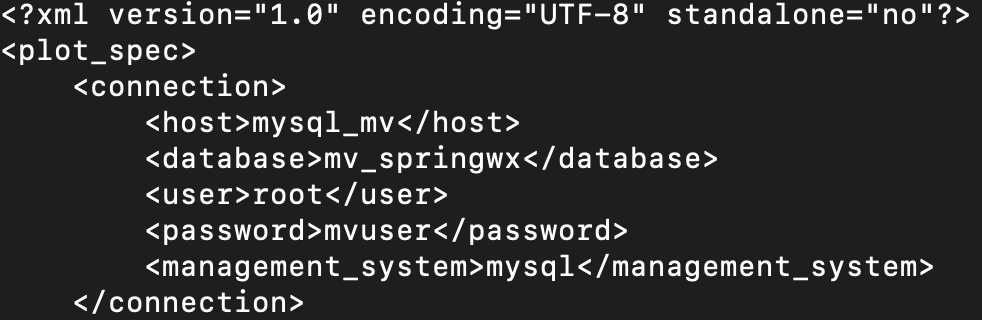
In addition, the other files can be modified based on the desired case specifics. For example, if you wish to change the variables being output in UPP, you will modify wrf_cntrl.parm (grib) or postcntrl.xml (grib2). If you are interested in changing variables, levels, or output types from MET, you will modify the MET configuration files under /met_config. More detailed information on the various components and their customization of WPS/WRF, UPP, and MET can be found in their respective User Guides:
With the scripts, namelists, and ancillary files ready for the new case, the next step is to retrieve the data for initial and boundary conditions, data assimilation, and verification.
Pulling data from AWS
Pulling data from AWSPulling data from Amazon S3 bucket
In this example, we will be retrieving 0.25° Global Forecast System (GFS) data from a publicly available Amazon Simple Storage Service (S3) bucket and storing it on our local filesystem, where it will be mounted for use in the Docker-space. The case is initialized at 00 UTC on 20210601 out to 24 hours in 3-hr increments.
To run the example case, first we need to set some variables and create directories that will be used for this specific example.
| tcsh | bash |
|---|---|
|
cd /home/ec2-user
setenv PROJ_DIR `pwd` setenv PROJ_VERSION 4.1.0
|
cd /home/ec2-user
export PROJ_DIR=`pwd` export PROJ_VERSION="4.1.0"
|
Then, you should set up the variables and directories for the experiment (spring_wx):
| tcsh | bash |
|---|---|
|
setenv CASE_DIR ${PROJ_DIR}/spring_wx
|
export CASE_DIR=${PROJ_DIR}/spring_wx
|
cd ${CASE_DIR}
mkdir -p wpsprd wrfprd gsiprd postprd pythonprd metprd metviewer/mysql
The GFS data needs to be downloaded into the appropriate directory, so we need to navigate to:
cd ${PROJ_DIR}/data/model_data/spring_wx
Next, run a script to pull GFS data for a specific initialization time (YYYYMMDDHH), maximum forecast length (HH), and increment of data (HH). For example:
If wget is not available on your system, an alternative is curl. You can, for example, modify the pull_aws_s3_gfs.ksh to have: curl -L -O
Run NWP initialization components (WPS, real.exe)
As with the provided canned cases, the first step in the NWP workflow will be to create the initial and boundary conditions for running the WRF model. This will be done using WPS and real.exe.
These commands are the same as the canned cases, with some case-specific updates to account for pointing to the appropriate scripts directory and name of the container.
SELECT THE APPROPRIATE CONTAINER INSTRUCTIONS FOR YOUR SYSTEM BELOW:
-v ${PROJ_DIR}/data/WPS_GEOG:/data/WPS_GEOG \
-v ${PROJ_DIR}/container-dtc-nwp/data:/data \
-v ${PROJ_DIR}/container-dtc-nwp/components/scripts/common:/home/scripts/common \
-v ${PROJ_DIR}/container-dtc-nwp/components/scripts/spring_wx:/home/scripts/case \
-v ${CASE_DIR}/wpsprd:/home/wpsprd \
--name run-springwx-wps dtcenter/wps_wrf:${PROJ_VERSION} /home/scripts/common/run_wps.ksh
-v ${PROJ_DIR}/data:/data \
-v ${PROJ_DIR}/container-dtc-nwp/components/scripts/common:/home/scripts/common \
-v ${PROJ_DIR}/container-dtc-nwp/components/scripts/spring_wx:/home/scripts/case \
-v ${CASE_DIR}/wpsprd:/home/wpsprd \
-v ${CASE_DIR}/wrfprd:/home/wrfprd \
--name run-springwx-real dtcenter/wps_wrf:${PROJ_VERSION} /home/scripts/common/run_real.ksh1
| tcsh | bash |
|---|---|
|
setenv TMPDIR ${CASE_DIR}/tmp
|
export TMPDIR=${CASE_DIR}/tmp
|
Updating Software Versions
Updating Software VersionsUpdating software component versions
Several components of the end-to-end WRF-based containerized system still undergo regular updates and public releases to the community (WPS, WRF, MET, METviewer), while others are frozen (GSI and UPP for WRF). If you would like to change the version of a component defined in the code base you have pulled from the NWP container project GitHub repository you will need to change the Dockerfile for that component in the source code.
Go to the wps_wrf directory:
Edit the Dockerfile to update the version number for WRF and WPS on lines 9 and 10. For example:
ENV WPS_VERSION 4.3
Once the version has been updated, follow the instructions for option #2 to build the dtcenter/wps_wrf image from scratch using the appropriate version number in the image name.
Go to the MET directory:
Edit the Dockerfile to update the version number for MET on line 8. For example:
Once the version has been updated, follow the instructions for option #2 to build the dtcenter/nwp-container-met image from scratch using the appropriate version number in the image name.
Go to the METviewer directory:
Edit the Dockerfile to update the version number for METviewer on line 8. The versions of METcalcpy (Python version of statistics calculation) and METplotpy (packages for plotting in METplus) may also be updated on lines 9 and 10. For example:
ENV METCALCPY_GIT_NAME v1.0.0
ENV METPLOTPY_GIT_NAME v1.0.0
Once the version has been updated, follow the instructions for option #2 to build the dtcenter/nwp-container-metviewer image from scratch using the appropriate version number in the image name.
NWP components
NWP componentsThe following sections provide examples of different customizations for the NWP software components. These examples are not exhaustive and are provided to give guidance for some common ways these components are modified and customized for new cases.
Changing WRF Namelist
Changing WRF NamelistChanging namelist options in WRF
Perhaps you'd like to rerun WRF with a different namelist option by changing a physics scheme. In this case, you'll want to rerun the WRF and all downstream components (i.e., UPP, Python graphics, MET, and METviewer), but you may not need to rerun the WPS, GSI, or Real components. In this example, we will demonstrate how to modify and rerun a container by modifying the namelist.input without deleting local output from a previous run.
Go to the scripts directory for the desired case:
Edit the namelist.input to making your desired modifications. For this example, we will change mp_physics from 4 (WSM5) to 8 (Thompson). **More information on how to set up and run WRF can be found on the Users' Page: http://www2.mmm.ucar.edu/wrf/users/
mp_physics = 8,
Rerun the WRF container using the local changes made to the namelist.input file and modifying the local WRF output directory (note: you can rename wrfprd whatever you choose):
Select the appropriate container instructions for your system below:
-v ${PROJ_DIR}/container-dtc-nwp/components/scripts/common:/home/scripts/common \
-v ${PROJ_DIR}/container-dtc-nwp/components/scripts/sandy_20121027:/home/scripts/case \
-v ${CASE_DIR}/wpsprd:/home/wpsprd -v ${CASE_DIR}/gsiprd:/home/gsiprd -v ${CASE_DIR}/wrfprd_mp6:/home/wrfprd \
--name run-sandy-wrf dtcenter/wps_wrf:${PROJ_VERSION} /home/scripts/common/run_wrf.ksh
Modify model domain
Modify model domainModifying the WRF model domain
This example demonstrates how to modify the domain for the Sandy case, but these procedures can be used as guidance for any other case as well.
Changing the model domain requires modifying the WRF namelist.wps and namelist.input. For this example, let's say you want to make the original Sandy domain larger and shift it westward to include more land.
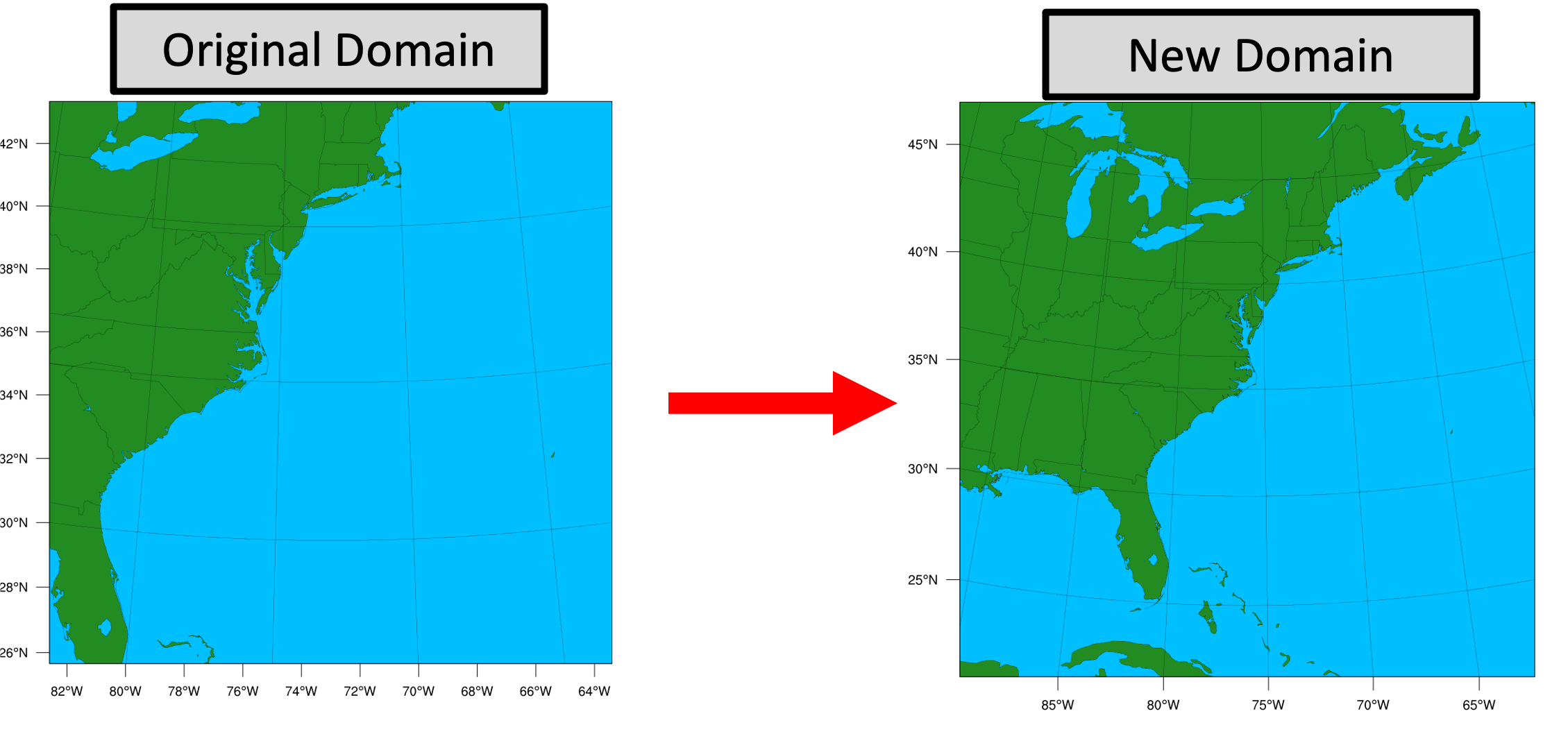
First, make sure you have created a new case directory so nothing is overwritten from the original run, and that your $CASE_DIR is properly set. See Setting Up a New Experiment
Next, modify the &geogrid section of the namelist.wps:
vi namelist.wps
Edits to &geogrid section of namelist.wps:
e_we: 50 --> 75 (line 15)
e_sn: 50 --> 75 (line 16)
ref_lon: -73. --> -76. (line 22)
stand_lon: -73.0 --> -76.0 (line 25)
The updated &geogrid section of the namelist.wps should look like this (with changes in bold):
parent_id = 1, 1,
parent_grid_ratio = 1, 3,
i_parent_start = 1, 31,
j_parent_start = 1, 17,
e_we = 75, 112,
e_sn = 75, 97,
geog_data_res = 'lowres', 'lowres',
dx = 40000,
dy = 40000,
map_proj = 'lambert',
ref_lat = 35.
ref_lon = -76.
truelat1 = 30.0,
truelat2 = 60.0,
stand_lon = -76.0,
geog_data_path = '/data/WPS_GEOG/',
opt_geogrid_tbl_path = '/comsoftware/wrf/WPS-4.1/geogrid',
/
The &domains section of the namelist.input file must also be updated to reflect these new domain parameters:
vi namelist.input
Edits to the &domains section of the namelist.input:
e_we: 50 --> 75 (line 38)
e_sn: 50 --> 75 (line 39)
time_step = 180,
time_step_fract_num = 0,
ime_step_fract_den = 1,
max_dom = 1,
e_we = 75, 112, 94,
e_sn = 75, 97, 91,
Now run the NWP components for your new case with the new domain.
SELECT THE APPROPRIATE CONTAINER INSTRUCTIONS FOR YOUR SYSTEM BELOW:
First run WPS:
Then run REAL:
Then run WRF:
-v ${PROJ_DIR}/container-dtc-nwp/components/scripts/common:/home/scripts/common \
-v ${PROJ_DIR}/container-dtc-nwp/components/scripts/sandy_20121027:/home/scripts/case \
-v ${CASE_DIR}/wpsprd:/home/wpsprd -v ${CASE_DIR}/gsiprd:/home/gsiprd -v ${CASE_DIR}/wrfprd:/home/wrfprd \
--name run-sandy-wrf dtcenter/wps_wrf:${PROJ_VERSION} /home/scripts/common/run_wrf.ksh
And continue running the remaining NWP components (i.e. UPP, MET, etc.)
First run WPS:
Then run REAL:
Then run WRF:
And continue running the remaining NWP components (i.e. UPP, MET, etc.)
Running WRF on multiple nodes with Singularity
Running WRF on multiple nodes with SingularityOne of the main advantages of Singularity is its broad support for HPC applications, specifically its lack of root privilege requirements and its support for scalable MPI on multi-node machines. This page will give an example of the procedure for running this tutorial's WPS/WRF Singularity container on multiple nodes on the NCAR Cheyenne supercomputer. The specifics of running on your particular machine of interest may be different, but you should be able to apply the lessons learned from this example to any HPC platform where Singularity is installed.
Step-by-step instructions
Load the singularity, gnu, and openmpi modules
module load gnu
module load openmpi
Set up experiment per usual (using snow case in this example)
git clone git@github.com:NCAR/container-dtc-nwp -b v${PROJ_VERSION}
mkdir data/ && cd data/
| tcsh | bash |
|---|---|
|
foreach f (/glade/p/ral/jntp/NWP_containers/*.tar.gz)
tar -xf "$f" end |
for f in /glade/p/ral/jntp/NWP_containers/*.tar.gz; do tar -xf "$f"; done
|
mkdir -p ${CASE_DIR} && cd ${CASE_DIR}
mkdir -p wpsprd wrfprd gsiprd postprd pythonprd metprd metviewer/mysql
export TMPDIR=${CASE_DIR}/tmp
mkdir -p ${TMPDIR}
Pull singularity image for wps_wrf from DockerHub
The Singularity containers used in this tutorial take advantage of the ability of the software to create Singularity containers from existing Docker images hosted on DockerHub. This allows the DTC team to support both of these technologies without the additional effort to maintain a separate set of Singularity recipe files. However, as mentioned on the WRF NWP Container page, the Docker containers in this tutorial contain some features (a so-called entrypoint script) to mitigate permissions issues seen with Docker on some platforms. Singularity on multi-node platforms does not work well with this entrypoint script, and because Singularity does not suffer from the same permissions issues as Docker, we have provided an alternate Docker container for use with Singularity to avoid these issues across multiple nodes:
Create a sandbox so the container is stored on disk rather than memory/temporary disk space
In the main tutorial, we create Singularity containers directly from the Singularity Image File (.sif). For multi-node Singularity, we will take advantage of an option known as "Sandbox" mode:
This creates a directory named "wps_wrf" that contains the entire directory structure of the singularity image; this is a way to interact with the Singularity container space from outside the container rather than having it locked away in the .sif file. You can use the ls command to view the contents of this directory, you will see it looks identical to the top-level directory structure of a typical linux install:
total 75
drwxr-xr-x 18 kavulich ral 4096 Feb 8 13:49 .
drwxrwxr-x 11 kavulich ral 4096 Feb 8 13:49 ..
-rw-r--r-- 1 kavulich ral 12114 Nov 12 2020 anaconda-post.log
lrwxrwxrwx 1 kavulich ral 7 Nov 12 2020 bin -> usr/bin
drwxr-xr-x 4 kavulich ral 4096 Feb 8 12:33 comsoftware
drwxr-xr-x 2 kavulich ral 4096 Feb 8 13:49 dev
lrwxrwxrwx 1 kavulich ral 36 Feb 8 13:42 environment -> .singularity.d/env/90-environment.sh
drwxr-xr-x 57 kavulich ral 16384 Feb 8 13:42 etc
lrwxrwxrwx 1 kavulich ral 27 Feb 8 13:42 .exec -> .singularity.d/actions/exec
drwxr-xr-x 4 kavulich ral 4096 Feb 8 12:52 home
lrwxrwxrwx 1 kavulich ral 7 Nov 12 2020 lib -> usr/lib
lrwxrwxrwx 1 kavulich ral 9 Nov 12 2020 lib64 -> usr/lib64
drwxr-xr-x 2 kavulich ral 4096 Apr 10 2018 media
drwxr-xr-x 2 kavulich ral 4096 Apr 10 2018 mnt
drwxr-xr-x 3 kavulich ral 4096 Dec 27 15:32 opt
drwxr-xr-x 2 kavulich ral 4096 Nov 12 2020 proc
dr-xr-x--- 5 kavulich ral 4096 Dec 27 16:00 root
drwxr-xr-x 13 kavulich ral 4096 Dec 27 16:20 run
lrwxrwxrwx 1 kavulich ral 26 Feb 8 13:42 .run -> .singularity.d/actions/run
lrwxrwxrwx 1 kavulich ral 8 Nov 12 2020 sbin -> usr/sbin
lrwxrwxrwx 1 kavulich ral 28 Feb 8 13:42 .shell -> .singularity.d/actions/shell
lrwxrwxrwx 1 kavulich ral 24 Feb 8 13:42 singularity -> .singularity.d/runscript
drwxr-xr-x 5 kavulich ral 4096 Feb 8 13:42 .singularity.d
drwxr-xr-x 2 kavulich ral 4096 Apr 10 2018 srv
drwxr-xr-x 2 kavulich ral 4096 Nov 12 2020 sys
lrwxrwxrwx 1 kavulich ral 27 Feb 8 13:42 .test -> .singularity.d/actions/test
drwxrwxrwt 7 kavulich ral 4096 Feb 8 12:53 tmp
drwxr-xr-x 13 kavulich ral 4096 Nov 12 2020 usr
drwxr-xr-x 18 kavulich ral 4096 Nov 12 2020 var
You can explore this directory to examine the contents of this container, but be cautious not to make any modifications that could cause problems later down the road!
Run WPS as usual
The command for running WPS is similar to that used in the main tutorial. Specifically, the fact that we are using a sandbox rather than creating a container straight from the singularity image file, requires a change to the run command. Note the bold part that is different from the original tutorial:
Prepare the wrfprd directory
Now this part is still a little hacky...but this will be cleaned up in future versions. Enter the wrfprd directory and manually link the met_em output files from WPS and rename them to the proper "nocolons" convention. Then, link in the contents of the WRF run directory containing the static input files and compiled executables from the container we created in a sandbox, and replace the default namelist with our case's custom namelist:
ln -sf ${CASE_DIR}/wps_wrf/comsoftware/wrf/WRF-4.3/run/* .
rm namelist.input
cp $PROJ_DIR/container-dtc-nwp/components/scripts/snow_20160123/namelist.input .
Finally, request as many cores/nodes as you want, reload the environment on compute nodes, and run!
qsub -V -I -l select=2:ncpus=36:mpiprocs=36 -q regular -l walltime=02:00:00 -A P48503002
ln -sf ${CASE_DIR}/wpsprd/met_em.* .
|
tcsh |
bash |
|---|---|
|
foreach f ( met_em.* )
setenv j `echo $f | sed s/\:/\_/g` mv $f $j end |
for f in met_em.*; do mv "$f" "$(echo "$f" | sed s/\:/\_/g)"; done
|
mpiexec -np 72 singularity run -u -B/glade:/glade ${CASE_DIR}/wps_wrf ./wrf.exe
The rest of the tutorial can be completed as normal.
Post Processing
Post ProcessingAdding a new output variable to UPP
Perhaps you would like to output a variable in WRF and UPP that is not part of the "out of the box" configuration provided with the tutorial cases. In this example, we will demonstrate how to modify the WRF namelist.input and UPP control files to output maximum updraft helicity. Note: This variable has already been added for the tutorial cases, but the steps provide a roadmap for other variables.
Go to the scripts directory for the desired case. In this example, we will be using the derecho case:
In order to output maximum updraft helicity, you will need to edit the WRF namelist.input by setting nwp_diagnostics = 1 under the time_control section in the namelist.input. See below for what this entry looks like:
run_days = 0,
run_hours = 24,
.
.
.
nwp_diagnostics = 1
/
For more information on the nwp_diagnostics package, please see the WRF documentation. Once the local changes to the namelist.input have been made, run WRF per the instructions in the tutorial. If the changes were successfully executed, you should see the UP_HELI_MAX variable in the WRF output.
Changes to the UPP control files are necessary to output maximum updraft helicity in the post-processed GRIB2 files. More extensive descriptions are provided in the UPP User's Guide, but the necessary steps will be briefly outlined below.
First, if you are not still in the scripts directory, navigate there:
The new variable needs to be added to the postcntrl.xml file, which is a file composed of a series of parameter blocks specifying the variables, fields, and levels. To add maximum helicity, add the following block (note: order in the file does not matter as long as the variables are within the </paramset> and </postxml> tags):
<shortname>MAX_UPHL_ON_SPEC_HGT_LVL_ABOVE_GRND_2-5km</shortname>
<pname>MXUPHL</pname>
<table_info>NCEP</table_info>
<scale>-3.0</scale>
</param>
Information on the specifics of populating the parameter blocks is available in the UPP User's Guide. Once the postcntrl.xml file is updated, additional control files need to be modified.
Due to software requirements, these changes need to be made using the UPP code directory that lives in the UPP container. To enter the container,
SELECT THE APPROPRIATE CONTAINER INSTRUCTIONS FOR YOUR SYSTEM BELOW:
To enter the Docker container, execute the following command:
-v ${PROJ_DIR}/container-dtc-nwp/components/scripts/derecho_20120629:/home/scripts/case \
--name run-derecho-upp dtcenter/upp:3.5.1 /bin/bash
All changes that need to be made will be under the UPP parm directory. First, the necessary control files need to be copied into the parm directory:
cp /home/scripts/case/post*xml .
An optional step to ensure the user-edited XML stylesheets (EMC_POST_CTRL_Scheme.xsd and EMC_POST_Avblflds_Scheme.xsd) are error free is to validate the postcntrl.xml and postavblflds.xml files. If the validation is successful, confirmation will be given (e.g., postcntrl.xml validates). Otherwise, it will return error messages. To run the optional validation step:
xmllint --noout --schema EMC_POST_Avblflds_Schema.xsd post_avblflds.xml
Once the XMLs are validated, the user will need to generate the flat file. Edit the makefile_comm to point to the full path of the parm directory in container space. The makefile_comm will call the perl program POSTXMLPreprocessor.pl to generate the flat file, postxconfig-NT_WRF.txt. Modify the makefile_comm to change the path of FLATFILEDIR and FLATFILENAME:
FLATFILENAME = postxconfig-NT_WRF.txt
To generate the flat file type:
make
If a new flat file is successfully generated, you will see a message "Flat file is new generated." In order to save the postxconfig-NT_WRF.txt file outside of the container, we need to move it to the directory in container space that is mounted to your local scripts directory. After that is complete, you can exit the container.
exit
After completing these steps, rerun the WRF and UPP steps as usual with Docker commands.
To enter the Singularity container, we can leverage the "sandbox" feature and make the changes locally. Execute the following command:
singularity build --sandbox upp_3.5.1 ${CASE_DIR}/upp_3.5.1.sif
This will create a directory called "upp_3.5.1" in your ${PROJ_DIR}. We can now go into that directory and leverage the already built UPP code to make the necessary changes.
cp ${PROJ_DIR}/dtc-nwp-container/components/scripts/derecho_20120629/post*xml .
An optional step to ensure the user-edited XML stylesheets (EMC_POST_CTRL_Scheme.xsd and EMC_POST_Avblflds_Scheme.xsd) are error free is to validate the postcntrl.xml and postavblflds.xml files. If the validation is successful, confirmation will be given (e.g., postcntrl.xml validates). Otherwise, it will return error messages. To run the optional validation step:
xmllint --noout --schema EMC_POST_Avblflds_Schema.xsd post_avblflds.xml
Once the XMLs are validated, the user will need to generate the flat file. Edit the makefile_comm to point to the full path of the parm directory in container space. The makefile_comm will call the perl program POSTXMLPreprocessor.pl to generate the flat file, postxconfig-NT_WRF.txt. Modify the makefile_comm to change the path of FLATFILEDIR and FLATFILENAME:
FLATFILENAME = postxconfig-NT_WRF.txt
To generate the flat file type:
make
If a new flat file is successfully generated, you will see a message "Flat file is new generated." We then want to make sure to copy this new postxconfig-NT_WRF.txt file to the local case scripts directory to ensure it is used.
Rerun WRF using the wps_wrf_3.5.1.sif as in the Derecho tutorial (note for this example we assume you're `pwd` is ${PROJ_DIR}:
Finally, run UPP using the "sandbox" Singularity container:
Some final notes on adding a new output variable with WRF and/or UPP:
-
In the official WRF release, maximum updraft helicity is already enabled to be output via the WRF Registry files. All that is needed to be available in the WRF output files is to modify the namelist.input by setting nwp_diagnostics = 1. If you need to modify the WRF Registry file, please contact us for assistance.
-
In the official UPP release, maximum updraft helicity is already a supported variable. While a large number of variables are supported, not all variables are written out. The original postcntrl.xml did not specify outputting maximum updraft helicity; therefore, modifications were made to add the variable to output. To add a new variable that is not available in UPP and to access a list of fields produced by UPP, please see the UPP User's Guide.
Graphics
GraphicsThis tutorial uses Python to visualize the post-processed model output. If users are familiar with Python, they may modify existing examples and/or create new plot types. As a note, while this tutorial supports plotting post-processed model output after running UPP, Python is also able to directly plot the NetCDF output from WRF (with numerous examples available online). Two customization options are provided below -- one for modifying the provided Python scripts and one for adding a new output variable to plot.
Modifying the provided Python script(s)
Users may modify existing script(s) by navigating to the /scripts/common directory and modifying the existing ALL_plot_allvars.py script (or the individual Python scripts). There are innumerable permutations for modifying the graphics scripts, based on user preferences, so one example will be chosen to show the workflow for modifying the plots. In this example, we will modify the ALL_plot_allvars.py script to change the contour levels used for plotting sea-level pressure.
Since the Hurricane Sandy case exceeds the current minimum value in the specified range, we will add 4 new contour levels. First, navigate to the Python plotting scripts directory:
vi ALL_plot_allvars.py
Edit the ALL_plot_allvars.py script to make the desired changes to the contour levels. For this example, we will be modifying line 466 from:
To extend the plotted values starting from 960 hPa:
After the new contour levels have been added, the plots can be generated using the same run command that is used for the supplied cases. Since we are interested in the impacts on the Hurricane Sandy plots, we will use the following run command:
-v ${PROJ_DIR}/container-dtc-nwp/components/scripts/common:/home/scripts/common \
-v ${PROJ_DIR}/container-dtc-nwp/components/scripts/sandy_20121027:/home/scripts/case \
-v ${PROJ_DIR}/data/shapefiles:/home/data/shapefiles \
-v ${CASE_DIR}/postprd:/home/postprd -v ${CASE_DIR}/pythonprd:/home/pythonprd \
--name run-sandy-python dtcenter/python:${PROJ_VERSION} /home/scripts/common/run_python.ksh
Adding a new plot type
In addition to modifying the ALL_plot_allvars.py for the current supported variables, users may want to add new variables to plot. The Python scripts use the pygrib module to read GRIB2 files. In order to determine what variables are available in the post-processed files and their names as used by pygrib, a simple script, read_grib.py, under the /scripts/common directory, is provided to print the variable names from the post-processed files. For this example, we will plot a new variable, wind at 850 hPa. This will require us to run the read_grib.py script to determine the required variable name. In order to run read_grib.py, we are assuming the user does not have access to Python and the necessary modules, so we will use the Python container. To enter the container, execute the following command:
-v ${PROJ_DIR}/container-dtc-nwp/components/scripts/common:/home/scripts/common \
-v ${PROJ_DIR}/container-dtc-nwp/components/scripts/sandy_20121027:/home/scripts/case \
-v ${PROJ_DIR}/data/shapefiles:/home/data/shapefiles \
-v ${CASE_DIR}/postprd:/home/postprd -v ${CASE_DIR}/pythonprd:/home/pythonprd \
--name run-sandy-python dtcenter/python:${PROJ_VERSION} /bin/bash
Once "in" the container, navigate to the location of the read_grib.py script and open the script:
vi read_grib.py
This script reads a GRIB2 file output from UPP, so this step does require that the UPP step has already been run. To execute the script:
For the standard output from the Hurricane Sandy case, here is the output from executing the script:
After perusing the output, you can see that the precipitable water variable is called 'Precipitable water.' To add the new variable to the ALL_plot_allvars.py script, it is easiest to open the script and copy the code for plotting a pre-existing variable (e.g., composite reflectivity) and modify the code for precipitable water:
In the unmodified ALL_plot_allvars.py script, copy lines 367-368 for reading in composite reflectivity, paste right below, and change the variable to be for precipitable water, where 'Precipitable water' is variable name obtained from the output of the read_grib.py:
![]()
Next, we will add a new code block for plotting precipitable water, based on copying, pasting, and modifying from the composite reflectivity block above it (lines 731-760 in the unmodified code):
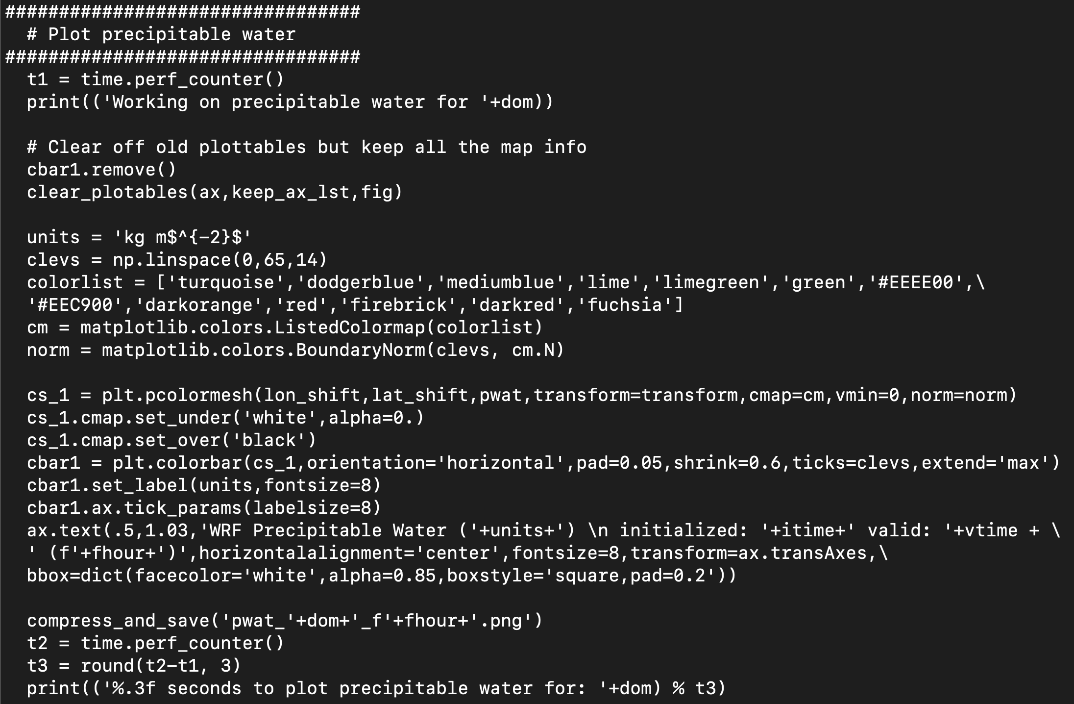
Note: This is a simple example of creating a new plot from the UPP output. Python has a multiple of customization options, with changes to colorbars, color maps, etc. For further customization, please refer to online resources.
To generate the new plot type, point to the scripts in the local scripts directory, run the dtcenter/python container to create graphics in docker-space and map the images into the local pythonprd directory:
-v ${PROJ_DIR}/container-dtc-nwp/components/scripts/common:/home/scripts/common \
-v ${PROJ_DIR}/container-dtc-nwp/components/scripts/sandy_20121027:/home/scripts/case \
-v ${PROJ_DIR}/data/shapefiles:/home/data/shapefiles \
-v ${CASE_DIR}/postprd:/home/postprd -v ${CASE_DIR}/pythonprd:/home/pythonprd \
--name run-sandy-python dtcenter/python:${PROJ_VERSION} /home/scripts/common/run_python.ksh
After Python has been run, the plain image output files will appear in the local pythonprd directory.
Here is an example of resulting plot of the precipitable water:
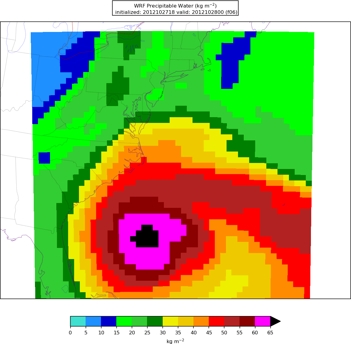
Verification
VerificationThe Model Evaluation Tools (MET) package includes many tools for forecast verification. More detailed information about MET can be found at the MET User's Page. The following MET tools are run by the /scripts/common/run_met.ksh shell script:
- PB2NC : pre-processes point observations from PREPBUFR files
- Point-Stat : verifies model output against point observations
- PCP-Combine : modifies precipitation accumulation intervals
- Grid-Stat : verifies model output against gridded analyses
The processing logic for these tools is specified by ASCII configuration files. Take a look at one of these configuration files:
- ${PROJ_DIR}/container-dtc-nwp/components/scripts/sandy_20121027/met_config/PointStatConfig_ADPSFC
Here you could add to or subtract from the list of variables to be verified. You could change the matching observation time window, modify the interpolation method, choose different output statistic line types, or make any number of other modifications. After modifying the MET configuration, rerunning the Docker run command for the verification component will recreate the MET output.
Database and display
Database and displayThe METviewer database and display system provides a flexible and interactive interface to ingest and visualize the statistical output of MET. In this tutorial, we loaded the MET outputs for each of the 3 supported case into separate databases named mv_derecho, mv_sandy, and mv_snow, which required running METviewer separately for each case by pointing to the specific ${CASE_DIR} directory. While sometimes it is desirable for each case to have its own database within a single METviewer instance, sometimes it is advantageous to load MET output from multiple cases into the same METviewer instance. For example, if a user had multiple WRF configurations they were running over one case, and they wanted to track the performance of the different configurations, they could load both case outputs into METviewer and analyze them together. The customization example below demonstrates how to load MET output from multiple cases into a METviewer database.
Load MET output from multiple cases into a METviewer database
In this example, we will execute a series of three steps: 1) reorganize the MET output from multiple cases to live under a new, top-level directory, 2) launch the METviewer container, using a modified Docker compose YML file, and 3) execute a modified METviewer load script to load the data into the desired database. For example purposes, we will have two cases: sandy (supplied, unmodified sandy case from the tutorial) and sandy_mp8 (modified sandy case to use Thompson microphysics, option 8); these instructions will only focus on the METviewer steps, assuming the cases have been run through the step to execute MET and create verification output.
Step 1: Reorganize the MET output
In order to load MET output from multiple cases in a METviewer database, the output must be rearranged from its original directory structure (e.g., $PROJ_DIR/sandy) to live under a new, top-level cases directory (e.g., $PROJ_DIR/cases/sandy). In addition, a new, shared metviewer/mysql directory must also be created.
mkdir -p $PROJ_DIR/metviewer/mysql
Once the directories are created, the MET output needs to be copied from the original location to the new location.
cp -r $PROJ_DIR/sandy_mp8/metprd/* $PROJ_DIR/cases/sandy_mp8
Step 2: Launch the METviewer container
In order to visualize the MET output from multiple cases using the METviewer database and display system, you first need to launch the METviewer container. These modified YML files differ from the original files used in the supplied cases by modifying the volume mounts to no longer be case-specific (i.e., use $CASE_DIR).
| FOR NON-AWS: | FOR AWS: |
|---|---|
|
|
|
Step 3: Load MET output into the database(s)
The MET output then needs to be loaded into the MySQL database for querying and plotting by METviewer by executing the load script (metv_load_cases.ksh), which requires three command line arguments: 1) name of database to load MET output (e.g., mv_cases), 2) path in Docker space where the case data will be mapped, which will be /data/{name of case directory used in Step 1}, and 3) whether you want a new database to load MET output into (YES) or load MET output into a pre-existing database (NO). In this example, where we have sandy and sandy_mp8 output, the following commands would be issued:
docker exec -it metviewer /scripts/common/metv_load_cases.ksh mv_cases /data/sandy_mp8 NO
The METviewer GUI can then be accessed with the following URL copied and pasted into your web browser:
Note, if you are running on AWS, run the following commands to reconfigure METviewer with your current IP address and restart the web service:
|
docker exec -it metviewer /bin/bash
/scripts/common/reset_metv_url.ksh exit |
The METviewer GUI can then be accessed with the following URL copied and pasted into your web browser (where IPV4_public_IP is your IPV4Public IP from the AWS “Active Instances” web page):
http://IPV4_public_IP/metviewer/metviewer1.jsp
These commands would load sandy and sandy_mp8 MET output into the mv_cases database. An example METviewer plot using sandy sandy_mp8 MET output is shown below (click here for XML used to create the plot).
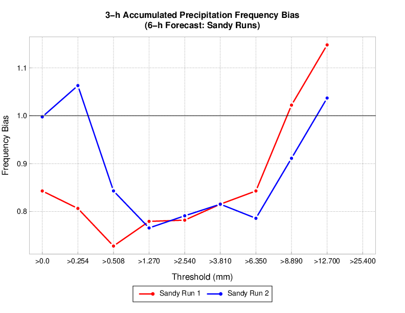
Modifying a container image
Modifying a container imageCurrently, procedures for this feature are only provided for Docker containers.
There may be a desire to make a change within a Docker container image and then use that updated image in an experiment. For example, you could make changes to the source code of a component, or modify default tables of a software component, etc. You The command docker commit allows one to save changes made within an existing container to a new image for future use.
In this example, we'll modify the wps_wrf container. Assuming you already have the wps_wrf:4.0.0 image pulled from Dockerhub (4.0.0. being the previously set ${PROJ_VERSION} variable), you should see your images following the docker images command. For example:
dtcenter/wps_wrf 4.0.0 3d78d8d63aec 2 months ago 3.81GB
We will deploy the container similar to running a component in our example cases, however with a few key difference. First, we'll omit the "--rm" option from the command so that when we exit the container it is not removed from our local list of containers and the changes persist in a local container. For simplicity, we'll also omit the mounting of local directories. Finally, we'll substitute our typical run command from a provided script to a simple /bin/bash. This allows us to enter the container in a shell environment to make changes and test any modifications.
[comuser@d829d8d812d6 wrf]$
Note the change in command prompt to something similar to: [comuser@d829d8d812d6 wrf]$, highlighting that you are now inside the container, and not on your local machine space. Do an "ls" to list what's in this container:
WPS-4.3 WRF WRF-4.3
Inside the container, you can now make any edits you want. You could make an edit to the WRF or WPS source code and recompile the code, or your make edits to predefined tables. For the purposes of illustrating the general concept of docker commit, we'll just add a text file in the container so we can see how to make it persist in a new image.
ls
Now exit the container.
You are now back on your local command line. List your containers to find the name of the container that you just modified and exited:
d829d8d812d6 dtcenter/wps_wrf:4.0.0 "/usr/local/bin/entr…" 33 seconds ago Exited (0) 20 seconds ago sweet_moser
Note the container d829d8d812d6 that we just exited. This is the container name id that we'll use to make a new image. Use docker commit to create a new image from that modified container. The general command is:
docker commit CONTAINER_ID_NAME NEW_IMAGE_NAME
So in this example:
Execute a docker images command to list your images and see the new image name.
wps_wrf_testfile latest f490d863a392 3 seconds ago 3.81GB
dtcenter/wps_wrf 4.0.0 3d78d8d63aec 2 months ago 3.81GB
You can deploy this new image and enter the container via a shell /bin/bash command to confirm this new image has your changes, e.g.:
useradd: user 'user' already exists
[comuser@05e6fb4618dd wrf]$
In the container, now do a "ls" to list the contents and see the test file.
Exit the container.
Once you have this new image, you can use it locally as needed. You could also push it to a Dockerhub repository where it will persist beyond your local machine and enable you to use docker pull commands and share the new image if needed.
Publicly Available Data Sets
Publicly Available Data SetsPublicly Available Data Sets
There are a number of publicly available data sets that can be used for initial and boundary conditions, data assimilation, and verification:
A list of the NOAA Big Data Program Datasets can be found here: https://www.noaa.gov/organization/information-technology/list-of-big-data-program-datasets
Model forecast data sets:
-
NOMADS: https://nomads.ncep.noaa.gov/pub/data/nccf/com/{model}/prod, where model may be:
-
GFS (grib2 or nemsio) - available for the last 10 days https://nomads.ncep.noaa.gov/pub/data/nccf/com/gfs/prod/
-
NAM - available for the last 8 days https://nomads.ncep.noaa.gov/pub/data/nccf/com/nam/prod/
-
RAP - available for the last 2 days https://nomads.ncep.noaa.gov/pub/data/nccf/com/rap/prod/
-
HRRR - available for the last 2 days https://nomads.ncep.noaa.gov/pub/data/nccf/com/hrrr/prod/
-
-
NCEI archive
-
AWS S3:
-
HRRR: https://registry.opendata.aws/noaa-hrrr-pds/ (necessary fields for initializing available for dates 2015 and newer)
-
Google Cloud:
-
Others:
-
Univ. of Utah HRRR archive: http://home.chpc.utah.edu/~u0553130/Brian_Blaylock/cgi-bin/hrrr_download.cgi
-
NAM nest archive: https://www.ready.noaa.gov/archives.php
-
NAM data older than 6 months can be requested through the Archive Information Request System: https://www.ncei.noaa.gov/has/HAS.FileAppRouter?datasetname=NAM218&subqueryby=STATION&applname=&outdest=FILE
-
RAP isobaric data older than 6 months can be requested through the Archive Information Request System: https://www.ncei.noaa.gov/has/HAS.FileAppRouter?datasetname=RAP130&subqueryby=STATION&applname=&outdest=FILE
-
Gridded precipitation data sets:
-
NCEP National StageIV Precipitation Analysis data
-
NCEP NOMADS Site: https://nomads.ncep.noaa.gov/pub/data/nccf/com/pcpanl/prod/
-
Past 14 days
-
-
NCEP FTP Site: ftp://ftp.emc.ncep.noaa.gov/mmb/sref/st2n4.arch
-
NCAR EOL Site: https://data.eol.ucar.edu/dataset/21.093
-
-
Multi-Radar/Multi-Sensor (MRMS) System Analysis data: https://mrms.ncep.noaa.gov/data/
-
Two day archive of precipitation, radar, and aviation and severe weather fields
-
-
Climatology-Calibrated Precipitation Analysis: https://ftp.ncep.noaa.gov/data/nccf/com/ccpa/prod/
-
8 days of most recent data
-
Prepbufr point observations:
-
AWS S3:
-
NCEP NOMADS Site:
-
PrepBufr for GDAS (Global): http://nomads.ncep.noaa.gov/pub/data/nccf/com/gfs/prod
-
10 days of most recent data
-
Data: gdas.YYYYMMDD/HH/gdas.tHHz.prepbufr.nr
-
-
PrepBufr for RAP (CONUS): http://nomads.ncep.noaa.gov/pub/data/nccf/com/rap/prod
-
1-2 days of most recent data
-
Data: rap.YYYYMMDD/rap.tHHz.prepbufr.tm00.nr
-
-
-
NCEP FTP Site:
-
PrepBufr for GDAS (Global): ftp://ftpprd.ncep.noaa.gov/pub/data/nccf/com/gfs/prod
-
10 days of most recent data
-
-
PrepBufr for NDAS (North America): ftp://ftpprd.ncep.noaa.gov/pub/data/nccf/com/rap/prod
-
1-2 days of most recent data
-
-
-
NCAR CISL Site:
-
DS337.0: NCEP PrepBufr ADP Global Upper Air and Surface Observations - archive starting May 1997
-
DS337.0 Subset: Interactive tool for running PB2NC over a specified time period and geographic region
-