METplus Practical Session Guide (July 2019)
METplus Practical Session Guide (July 2019)Welcome to the METplus Practical Session Guide
July 30 - August 1, 2019, at U.S. Naval Research Lab (NRL) in Monterey, California
The METplus practical consists of five sessions. Each session contains instructions for running individual MET tools directly on the command line followed by instructions for running the same tools as part of a METplus use case.
Please follow the link to the appropriate session:
- Session 1
METplus Setup/Grid-to-Grid - Session 2
Grid-to-Obs - Session 3
Ensemble and PQPF - Session 4
MODE and MTD - Session 5
Trk&Int/Feature Relative
The Tutorial Schedule contains PDF's of the lecture slides and final versions will be posted here after the tutorial.
Session 1: METplus Setup/Grid-to-Grid
Session 1: METplus Setup/Grid-to-Grid admin Wed, 06/12/2019 - 16:55METplus Practical Session 1
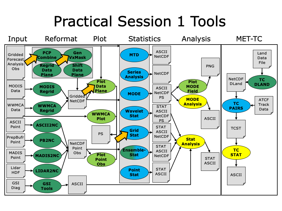
During the first METplus practical session, you will run the tools indicated below:
During this practical session, please work on the Session 1 exercises. Proceed through the tutorial exercises by following the navigation links at the bottom of each page.
Each practical session builds on the output of previous practical sessions. So please work on them in the order listed.
Throughout this tutorial, code blocks in BOLD white text with a black background should be copied from your browser and pasted on the command line. You can copy-and-paste the text using one of two methods:
- Use the mouse:
- Hold down the left mouse button to select the text
- Place the mouse in the desired location and click the middle mouse button once to paste the selected text
- Use the Copy and Paste options:
- Hold down the left mouse button to select the text
- Click the right mouse button and select the option for Copy
- Place the mouse in the desired location, click the right mouse button, and select the option for Paste
Note: Instructions in this tutorial use vi to open and edit files. If you prefer to use a different file editor, feel free to substitute it whenever you see vi.
Note: Instructions in this tutorial use okular to view pdf, ps, and png files. If you prefer to use a different file viewer, feel free to substitute it whenever you see okular.
Click the 'METplus Setup >' on the bottom right to get started!
METplus Setup
METplus Setup admin Mon, 06/24/2019 - 15:58METplus Overview
METplus is a set of python modules that have been developed with the flexibility to run MET for various use cases or scenarios. The goal is to simplify the running of MET for scientists. Currently, the primary means of achieving this is through the use of METplus configuration files, aka. "conf files". It is designed to provide a framework in which additional MET use cases can be added. The conf file implementation utilizes a Python package called produtil that was developed by NOAA/NCEP/EMC for the HWRF system.
The METplus Python application is designed to be run as stand alone module files - calling one MET process; through a user defined process list - as in this tutorial; or within a workflow management system on an HPC cluster - which is TBD.
Please be sure to follow the instructions in order.
METplus Useful Links
The following links are just for reference, and not required for this practical session. A METplus release is available on GitHub, and provides sample data and instructions.
GitHub METplus links
The METplus-related code repositories are available in GitHub in the following locations:
- https://github.com/NCAR/METplus - Python wrappers and use cases
- https://github.com/NCAR/MET - Core MET codebase
- https://github.com/NCAR/METviewer - Display system for MET output
- https://github.com/NCAR/METdb - Database system for MET output (currently private)
- https://github.com/NCAR/METplotpy - Python plotting scripts (currently private)
- https://github.com/NCAR/METcalcpy - Python calculation functions (currently private)
- METexpress - Streamlined display system (currently lives in NOAA's VLab)
New features are developed and bugs are tracked using GitHub issues in each repository.
METplus: Initial setup
METplus: Initial setup admin Mon, 06/24/2019 - 15:59Prequisites: Software
The following is a full list of software that is required to utilize all the functionality in METplus.
NOTE: We will not by running the cyclone plotter or grid plotting scripts in this tutorial. So the additional libraries mentioned below are not installed.
- Python 2.7.x
- Additional Python libraries: - required by the cyclone plotter and grid plotting scripts.
- numpy
- matplotlib - not installed, Is is not required for this tutorial.
- cartopy - not installed, It is not required for this tutorial.
- MET 8.1 - already installed locally on the tutorial machines.
- R - used by TCMPRPlotter wrapper, Wraps the MET plot_tcmpr.R script
- ncap2 - NCO netCDF Operators
- wgrib2 - only needed for series analysis wrappers (SeriesByLead and SeriesByInit)
- ncdump - NetCDF binaries
- convert - Utilitity from ImageMagick software suite
Prequisites: Environment
Before running these instructions, you will need to ensure that you have a few environment variables set up correctly. If they are not set correctly, these instructions will not work properly.
- Check that you have METPLUS_TUTORIAL_DIR set correctly:
If you don't see a path in your user directory output to the screen, set this environment variable in your user profile before continuing.
- Check that you have METPLUS_BUILD_BASE, MET_BUILD_BASE, and METPLUS_DATA set correctly:
echo ${MET_BUILD_BASE}
echo ${METPLUS_DATA}
If any of these variables are not set, please set them. They will be referenced throughout the tutorial.
MET_BUILD_BASE is the full path to the MET installation (/path/to/met-X.Y)
METPLUS_DATA is the location of the sample test data directory
- Check that you have loaded the MET module correctly:
You should see the usage statement for Point-Stat. The version number listed should correspond to the version listed in MET_BUILD_BASE. If it does not, you will need to either reload the met module, or add ${MET_BUILD_BASE}/bin to your PATH.
Getting The Software
For this tutorial we'll use the METplus v2.2 release, which has been installed in a common location. We will configure METplus to run the met-8.1 software, which has also been installed in a common location. We will copy the parameter files from the shared METplus location to your own directory so you can modify them without changing the shared installation settings.
Please use the following instructions to setup METplus on your tutorial machine:
- Create a directory to store your METplus files (include the version number for traceability):
- Create a symbolic link so that you can refer to the METplus directory instead of METplus-2.2 (you may need to remove the link if it already exists):
ln -s METplus-2.2 METplus
- List the contents of the metplus_tutorial directory:
You should see something similar to this:
drwxrwxr-x 2 mccabe rap 4096 Jul 18 15:34 METplus-2.2
- Copy the parm directory from the shared METplus location to your home directory:
- Create directory to store configuration files you will create:
For reference, the following are instructions to download and install METplus on your own machine.
- If you wish, download and unpack the release tarball and create a METplus symbolic link:
DO NOT RUN THESE COMMANDS FOR THE TUTORIAL!
wget https://github.com/NCAR/METplus/archive/v2.2.tar.gz
tar -xvzf METplus_v2.2.tar.gz
rm METplus
ln -s METplus-2.2 METplus
Sample Data Input and Location of Output
The Sample Input Data used to run the examples in this tutorial already exist in a shared location. For reference, here are example instructions to obtain the sample input data.
DO NOT RUN THESE COMMANDS FOR THE TUTORIAL!
cd /d1/METplus-2.2_Data
wget https://github.com/NCAR/METplus/releases/download/v2.2/sample_data-grid_to_grid-2.2.tgz
tar -xvzf sample_data-grid_to_grid-2.2.tgz
rm sample_data-grid_to_grid-2.2.tgz
This will create a directory named 'grid_to_grid' under '/d1/METplus_Data' that contains all of the sample input data needed to run the grid_to_grid use cases (found in parm/use_cases/grid_to_grid/examples). Other sample data tarballs are available under 'Assets' on the METplus GitHub releases page.
When running METplus wrapper use cases, all output is placed in the ${METPLUS_TUTORIAL_DIR}/output directory.
When running MET on the command line, all output will be written to ${METPLUS_TUTORIAL_DIR}/output/met_output
Your Runtime Environment
For this tutorial, the MET software is available via a module file. This has already been loaded for all users, so the MET software is available when you login.
The PATH environment variable is set to allow the METplus scripts to be run from any directory.
- Edit the .bash_profile file to configure your runtime environment for use with METplus:
Add the following at the end of the file to set the PATH and METPLUS_PARM_BASE environment variables. Also update LD_LIBRARY_PATH to avoid runtime NetCDF linker errors:
bash:
export METPLUS_PARM_BASE=${METPLUS_TUTORIAL_DIR}/METplus/parm
export LD_LIBRARY_PATH=/software/depot/met-8.1/external_libs/lib:${LD_LIBRARY_PATH}
csh:
setenv METPLUS_PARM_BASE ${METPLUS_TUTORIAL_DIR}/METplus/parm
setenv LD_LIBRARY_PATH /software/depot/met-8.1/external_libs/lib:${LD_LIBRARY_PATH}
Save and close that file, then source it to apply the settings to the current shell. The next time you login, you do not have to source this file again:
If you did everything correctly, running 'which master_metplus.py' should show you the path to the script in the shared location, ${METPLUS_BUILD_BASE}:
METplus: Directories and Configuration Files - Overview
METplus: Directories and Configuration Files - Overview admin Mon, 06/24/2019 - 15:59METplus directory structure
Brief description and overview of the METplus/ directory structure.
- doc/ - Doxygen files for building the html API documentation.
- doc/METplus_Users_Guide - LyX files and the user guide PDF file.
- internal_tests/ - for engineering tests
- parm/ - where config files live
- README.md - general README
- sorc/ - executables and documentation build system
- ush/ - python scripts
METplus default configuration files
The METplus default configuration files metplus_system.conf, metplus_data.conf, metplus_runtime.conf, and metplus_logging.conf are always read by default and in the order shown. Any additional configuration files passed in on the command line are than processed in the order in which they are specified. This allows for each successive conf file the ability to override variables defined in any previously processed conf files. It also allows for defining and setting up conf files from a general (settings used by all use cases, ie. MET install dir) to more specific (Plot type when running track and intensity plotter) structure. The idea is to created a hiearchy of conf files that is easier to maintain, read, and manage. It is important to note, running METplus creates a single configuration file, which can be viewed to understand the result of all the conf file processing.
The final metplus conf file is defined here:
metplus_runtime.conf:METPLUS_CONF={OUTPUT_BASE}/metplus_final.conf
Use this file to see the result of all the conf file processing, this can be very helpful when troubleshooting,
NOTE: The syntax for METplus configuration files MUST include a "[section]" header with the variable names and values on subsequent lines.
Unless otherwise indicated, all directories are relative to your ${METPLUS_PARM_BASE} directory.
The metplus_config directory - there are four config files:
- metplus_system.conf
- contains "[dir]" and "[exe]" to set directory and executable paths
- any information specific to host machine
- metplus_data.conf
- Sample data or Model input location
- filename templates and regex for filenames
- metplus_runtime.conf
- contains "[config]" section
- var lists, stat lists, configurations, process list
- anything else needed at runtime
- metplus_logging.conf
- contains "[dir]" section for setting the location of log files.
- contains "[config]" section for setting various logging configuration options.
The use_cases directory - The use cases:
This is where the use cases you will be running exist. The use case filenaming and directory structure is by convention. It is intended to simplify management of common configuration items for a specific use case. Under the use_cases directory is a subdirectory for each use case. Under that is an examples subdirectory and a more general configuration file that contains information that is shared by examples of the use case.
- For example, the track and intensity use case conf directory and file structure.
- track_and_intensity - directory
- track_and_intensity/track_and_intensity.conf - use case configuration file
- track_and_intensity/examples - directory to hold various track and intensity example conf files.
- track_and_intensity/examples/tcmpr_mean_median.conf - specific use case
- track_and_intensity/examples/README - File containing instructions to run the use case examples in this directory.
Within each use case there is a met_config subdirectory that contains MET specific config files for that use case. The use_cases/<use case>/met_config directory - store all your MET config files, e.g.:
- GridStatConfig_anom (for MET grid_stat)
- TCPairsETCConfig (for MET tc_pairs)
- SeriesAnalysisConfig_by_init (for MET series_analysis)
- SeriesAnalysisConfig_by_lead (for MET series_analysis)
METplus: User Configuration Settings
METplus: User Configuration Settings admin Mon, 06/24/2019 - 16:00Modify your METplus conf files
In this section you will modify the configuration files that will be read for each call to METplus.
The paths in this practical assume:
- You have copied the parm directory from the shared METplus location into your ${METPLUS_TUTORIAL_DIR}/METplus directory
- You have added the shared METplus ush directory to your PATH
- You have set the METPLUS_PARM_BASE environment variable to your copied parm directory
- You are using the shared installation of MET.
If not, then you need to adjust accordingly.
- Try running master_metplus.py. You should see the usage statement output to the screen.
- Now try to pass in the example.conf configuration file found in your parm directory under use_cases/wrappers/examples
You should see an error message stating that OUTPUT_BASE was not set correctly. You will need to configure the METplus wrappers to be able to run a use case.
The values in the default metplus_system.conf, metplus_data.conf, metplus_runtime.conf, and metplus_logging.conf configuration files are read in first when you run master_metplus.py. The settings in these files can be overridden in the use case conf files and/or a user's custom configuration file.
Some variables in the system conf are set to '/path/to' and must be overridden to run METplus, such as OUTPUT_BASE in metplus_system.conf.
- View the metplus_system.conf file and notice how OUTPUT_BASE = /path/to . This implies it is REQUIRED to be overridden to a valid path.
Note: The default installation of METplus has /path/to values for MET_INSTALL_DIR, TMP_DIR, and INPUT_BASE. These values were set in the shared METplus configuration when it was installed. This was done because these settings will likely be set to the same values for all users.
- Change directory to your ${METPLUS_PARM_BASE} directory and modify the METplus base configuration files using the editor of your choice (vi listed as an example).
If METPLUS_PARM_BASE is set correctly, you should now be in ${METPLUS_TUTORIAL_DIR}/METplus/parm/metplus_config
Note: A METplus conf file is not a shell script.
You CAN NOT refer to environment variables as you would in a shell script or command prompt, i.e. ${HOME}.
Instead, you must reference the environment variable $HOME as {ENV[HOME]}
Reminder: Make certain to maintain the KEY = VALUE pairs under their respective current [sections] in the conf file.
- Set the [dir] INPUT_BASE variable to the location of the METplus sample data that will be used in the exercises
- Set the [dir] OUTPUT_BASE variable to the location you will write output data
Set the [dir] MET_INSTALL_DIR variable to the location where MET is installed (this should already be done when METplus was installed in the shared location)
Set the [dir] TMP_DIR variable to a location you have write permissions
MET_INSTALL_DIR = {ENV[MET_BUILD_BASE]}
TMP_DIR = {OUTPUT_BASE}/tmp
NOTE: When installing METplus, you will need to set the full path to the non-MET executables in the metplus_system.conf file if they are not found in the user's path. This step was completed when METplus was installed in the shared location.
Creating user conf files
You can create additional configuration files to be read by the METplus wrappers to override variables.
Reminder: When adding variables to be overridden, make sure to place the variable under the appropriate section.
For example, [config], [dir], [exe]. If necessary, refer to the default appropriate parm/metplus_config conf files to determine the [section] that corresponds to the variable you are overriding. The value set will be the last one in the sequence of configuration files. See OUTPUT_BASE/metpus_final.conf to see what values were used for a given METplus run.
- Create a new configuration file in your user_config directory and override the [dir] OUTPUT_BASE variable to point to a different location.
vi change_output_base.conf
Copy and paste the following text into the file and save it.
OUTPUT_BASE = {ENV[METPLUS_TUTORIAL_DIR]}/output_changed
We will test out using these configurations on the next page.
METplus: How to Run
METplus: How to Run admin Mon, 06/24/2019 - 16:04Running METplus
Running METplus involves invoking the python script master_metplus.py followed by a list of configuration files using the -c option for each additional conf file.
Reminder: The default set of conf files are always read in and processed in the following order;
metplus_system.conf, metplus_data.conf, metplus_runtime.conf, metplus_logging.conf.
If you have configured METplus correctly and run master_metplus.py without passing in any configuration files, it will generate a usage statement to indicate that other config files are required to perform a useful task. It will generate an error statement if something is amiss.
- Review the example.conf configuration file
- Call the master_metplus.py script, passing in the example.conf configuration file with the -c command line option. You should see logs output to the screen.
Note: If master_metplus.py can't be found, you may need to add it to the path. Optionally, you can specify the full path to the script.
Note: The environment variable METPLUS_PARM_BASE determines where to look for relative paths to configuration files. If the environment variable is not set, the script will look in the parm directory that is associated with the version of master_metplus.py that is being called. Optionally, you can specify the full path to the configuration files.
OPTIONAL:
- Check the directory specified by the OUTPUT_BASE configuration variable. You should see that files and sub-directories have been created
- Review the master log file to see what was run. Compare the log output to the example.conf configuration file to see how they correspond to each other. The log file will have today's date in the filename
You will notice that METplus ran for 4 valid times, processing 4 forecast hours for each valid time. For each run, it used the input template to determine which file to look for.
- Now run METplus passing in the example.conf from the previous run AND your newly created configuration file.
- Check the directory specified by the OUTPUT_BASE configuration variable that you set in the change_output_base.conf configuration file. You should see that files and sub-directories have been created in the new location.
Remember: Additional conf files are processed after the metplus_config files in the order specified on the command line.
Order matters, since each successive conf file will override any variable defined in a previous conf file.
Note: The processing order allows for structuring your conf files from general (variables shared-by-all) to specific (variables shared-by-few).
MET Tool: PCP-Combine
MET Tool: PCP-Combine admin Mon, 06/24/2019 - 16:05We now shift to a dicussion of the MET PCP-Combine tool and will practice running it directly on the command line. Later in this session, we will run PCP-Combine as part of a METplus use case.
PCP-Combine Functionality
The PCP-Combine tool is used (if needed) to add, subtract, or sum accumulated precipitation from several gridded data files into a single NetCDF file containing the desired accumulation period. It's NetCDF output may be used as input to the MET statistics tools. PCP-Combine may be configured to combine any gridded data field you'd like. However, all gridded data files being combined must have already been placed on a common grid. The copygb utility is recommended for re-gridding GRIB files. In addition, the PCP-Combine tool will only sum model files with the same initialization time unless it is configured to ignore the initialization time.
PCP-Combine Usage
View the usage statement for PCP-Combine by simply typing the following:
| Usage: pcp_combine | ||
| [[-sum] sum_args] | [-add input_files] | [-subtract input_files] | [-derive stat_list input_files] (Note: "|" means "or") |
||
| [-sum] sum_args | Precipitation from multiple files containing the same accumulation interval should be summed up using the arguments provided. | |
| -add input_files | Data from one or more files should be added together where the accumulation interval is specified separately for each input file. | |
| -subtract input_files | Data from exactly two files should be subtracted. | |
| -derive stat_list input_files | The comma-separated list of statistics in "stat_list" (sum, min, max, range, mean, stdev, vld_count) should be derived using data from one or more files. | |
| out_file | Output NetCDF file to be written. | |
| [-field string] | Overrides the default use of accumulated precipitation (optional). | |
| [-name list] | Overrides the default NetCDF variable name(s) to be written (optional). | |
| [-log file] | Outputs log messages to the specified file | |
| [-v level] | Level of logging | |
| [-compress level] | NetCDF file compression |
Use the -sum, -add, or -subtract command line option to indicate the operation to be performed. Each operation has its own set of required arguments.
PCP-Combine Tool: Run Sum Command
PCP-Combine Tool: Run Sum Command admin Mon, 06/24/2019 - 16:13Since PCP-Combine performs a simple operation and reformatting step, no configuration file is needed.
- Start by making an output directory for PCP-Combine and changing directories:
cd ${METPLUS_TUTORIAL_DIR}/output/met_output/pcp_combine
- Now let's run PCP-Combine twice using some sample data that's included with the MET tarball:
-sum 20050807_000000 3 20050807_120000 12 \
sample_fcst_12L_2005080712V_12A.nc \
-pcpdir ${METPLUS_DATA}/met_test/data/sample_fcst/2005080700
-sum 00000000_000000 1 20050807_120000 12 \
sample_obs_12L_2005080712V_12A.nc \
-pcpdir ${METPLUS_DATA}/met_test/data/sample_obs/ST2ml
The "\" symbols in the commands above are used for ease of reading. They are line continuation markers enabling us to spread a long command line across multiple lines. They should be followed immediately by "Enter". You may copy and paste the command line OR type in the entire line with or without the "\".
Both commands run the sum command which searches the contents of the -pcpdir directory for the data required to create the requested accmululation interval.
In the first command, PCP-Combine summed up 4 3-hourly accumulation forecast files into a single 12-hour accumulation forecast. In the second command, PCP-Combine summed up 12 1-hourly accumulation observation files into a single 12-hour accumulation observation. PCP-Combine performs these tasks very quickly.
We'll use these PCP-Combine output files as input for Grid-Stat. So make sure that these commands have run successfully!
PCP-Combine Tool: Output
PCP-Combine Tool: Output admin Mon, 06/24/2019 - 16:13When PCP-Combine is finished, you may view the output NetCDF files it wrote using the ncdump and ncview utilities. Run the following commands to view contents of the NetCDF files:
ncview sample_obs_12L_2005080712V_12A.nc &
ncdump -h sample_fcst_12L_2005080712V_12A.nc
ncdump -h sample_obs_12L_2005080712V_12A.nc
The ncview windows display plots of the precipitation data in these files. The output of ncdump indicates that the gridded fields are named APCP_12, the GRIB code abbreviation for accumulated precipitation. The accumulation interval is 12 hours for both the forecast (3-hourly * 4 files = 12 hours) and the observation (1-hourly * 12 files = 12 hours).
Plot-Data-Plane Tool
The Plot-Data-Plane tool can be run to visualize any gridded data that the MET tools can read. It is a very helpful utility for making sure that MET can read data from your file, orient it correctly, and plot it at the correct spot on the earth. When using new gridded data in MET, it's a great idea to run it through Plot-Data-Plane first:
sample_fcst_12L_2005080712V_12A.nc \
sample_fcst_12L_2005080712V_12A.ps \
'name="APCP_12"; level="(*,*)";'
Next try re-running the command list above, but add the convert(x)=x/25.4; function to the config string (Hint: after the level setting but before the last closing tick) to change units from millimeters to inches. What happened to the values in the colorbar?
Now, try re-running again, but add the censor_thresh=lt1.0; censor_val=0.0; options to the config string to reset any data values less 1.0 to a value of 0.0. How has your plot changed?
The convert(x) and censor_thresh/censor_val options can be used in config strings and MET config files to transform your data in simple ways.
PCP-Combine Tool: Add and Subtract Commands
PCP-Combine Tool: Add and Subtract Commands admin Mon, 06/24/2019 - 16:14We have run examples of the PCP-Combine -sum command, but the tool also supports the -add, -subtract, and -derive commands. While the -sum command defines a directory to be searched, for -add, -subtract, and -derive we tell PCP-Combine exactly which files to read and what data to process. The following command adds together 3-hourly precipitation from 4 forecast files, just like we did in the previous step with the -sum command:
${METPLUS_DATA}/met_test/data/sample_fcst/2005080700/wrfprs_ruc13_03.tm00_G212 03 \
${METPLUS_DATA}/met_test/data/sample_fcst/2005080700/wrfprs_ruc13_06.tm00_G212 03 \
${METPLUS_DATA}/met_test/data/sample_fcst/2005080700/wrfprs_ruc13_09.tm00_G212 03 \
${METPLUS_DATA}/met_test/data/sample_fcst/2005080700/wrfprs_ruc13_12.tm00_G212 03 \
add_APCP_12.nc
By default, PCP-Combine looks for accumulated precipitation, and the 03 tells it to look for 3-hourly accumulations. However, that 03 string can be replaced with a configuration string describing the data to be processed. The configuration string should be enclosed in single quotes. Below, we add together the U and V components of 10-meter wind from the same input file. You would not typically want to do this, but this demonstrates the functionality. We also use the -name command line option to define a descriptive output NetCDF variable name:
${METPLUS_DATA}/met_test/data/sample_fcst/2005080700/wrfprs_ruc13_03.tm00_G212 'name="UGRD"; level="Z10";' \
${METPLUS_DATA}/met_test/data/sample_fcst/2005080700/wrfprs_ruc13_03.tm00_G212 'name="VGRD"; level="Z10";' \
add_WINDS.nc \
-name UGRD_PLUS_VGRD
While the -add command can be run on one or more input files, the -subtract command requires exactly two. Let's rerun the wind example from above but do a subtraction instead:
${METPLUS_DATA}/met_test/data/sample_fcst/2005080700/wrfprs_ruc13_03.tm00_G212 'name="UGRD"; level="Z10";' \
${METPLUS_DATA}/met_test/data/sample_fcst/2005080700/wrfprs_ruc13_03.tm00_G212 'name="VGRD"; level="Z10";' \
subtract_WINDS.nc \
-name UGRD_MINUS_VGRD
Now run Plot-Data-Plane to visualize this output. Use the -plot_range option to specify a the desired plotting range, the -title option to add a title, and the -color_table option to switch from the default color table to one that's good for positive and negative values:
subtract_WINDS.nc \
subtract_WINDS.ps \
'name="UGRD_MINUS_VGRD"; level="(*,*)";' \
-plot_range -15 15 \
-title "10-meter UGRD minus VGRD" \
-color_table ${MET_BUILD_BASE}/share/met/colortables/NCL_colortables/posneg_2.ctable
Now view the results:
PCP-Combine Tool: Derive Command
PCP-Combine Tool: Derive Command johnhg Tue, 07/23/2019 - 17:13While the PCP-Combine -add and -subtract commands compute exactly one output field of data, the -derive command can compute multiple output fields in a single run. This command reads data from one or more input files and derives the output fields requested on the command line (sum, min, max, range, mean, stdev, vld_count).
Run the following command to derive several summary metrics for both the 10-meter U and V wind components:
${METPLUS_DATA}/met_test/data/sample_fcst/2005080700/wrfprs_ruc13_*.tm00_G212 \
-field 'name="UGRD"; level="Z10";' \
-field 'name="VGRD"; level="Z10";' \
derive_min_max_mean_stdev_WINDS.nc
In the above example, we used a wildcard to list multiple input file names. And we used the -field command line option twice to specify two input fields. For each input field, PCP-Combine loops over the input files, derives the requested metrics, and writes them to the output NetCDF file. Run ncview to visualize this output:
This output file contains 8 variables: 2 input fields * 4 metrics. Note the output variable names the tool chose. You can still override those names using the -name command line argument, but you would have to specify a comma-separated list of 8 names, one for each output variable.
MET Tool: Gen-Vx-Mask
MET Tool: Gen-Vx-Mask admin Mon, 06/24/2019 - 16:06Gen-Vx-Mask Functionality
The Gen-Vx-Mask tool may be run to speed up the execution time of the other MET tools. Gen-Vx-Mask defines a bitmap masking region for your domain. It takes as input a gridded data file defining your domain and a second arguement to define the area of interest (varies by masking type). It writes out a NetCDF file containing a bitmap for that masking region. You can run Gen-Vx-Mask iteratively, passing its output back in as input, to define more complex masking regions.
You can then use the output of Gen-Vx-Mask to define masking regions in the MET statistics tools. While those tools can read ASCII lat/lon polyline files directly, they are able to process the output of Gen-Vx-Mask much more quickly than the original polyline. The idea is to define your masking region once for your domain with Gen-Vx-Mask and apply the output many times in the MET statistics tools.
Gen-Vx-Mask Usage
View the usage statement for Gen-Vx-Mask by simply typing the following:
| Usage: gen_vx_mask | ||
| input_file | Gridded data file defining the domain | |
| mask_file | Defines the masking region and varies by -type | |
| out_file | Output NetCDF mask file to be written | |
| [-type string] | Masking type: poly, box, circle, track, grid, data, solar_alt, solar_azi, lat, lon, shape | |
| [-input_field string] | Define field from input_file for grid point initialization values, rather than 0. | |
| [-mask_field string] | Define field from mask_file for data masking. | |
| [-complement, -union, -intersection, -symdiff] | Set logic for combining input_field initialization values with the current mask values. | |
| [-thresh string] | Define threshold for circle, track, data, solar_alt, solar_azi, lat, and lon masking types. | |
| [-height n, -width n] | Define dimensions for box masking. | |
| [-shapeno n] | Define the index of the shape for shapefile masking. | |
| [-value n] | Output mask value to be written, rather than 1. | |
| [-name str] | Specifies the name to be used for the mask. | |
| [-log file] | Outputs log messages to the specified file | |
| [-v level] | Level of logging | |
| [-compress level] | NetCDF compression level |
At a minimum, the input data_file, the input mask_poly polyline file, and the output netcdf_file must be passed on the command line.
Gen-Vx-Mask Tool: Run
Gen-Vx-Mask Tool: Run admin Mon, 06/24/2019 - 16:16Start by making an output directory for Gen-Vx-Mask and changing directories:
cd ${METPLUS_TUTORIAL_DIR}/output/met_output/gen_vx_mask
Since Gen-Vx-Mask performs a simple masking step, no configuration file is needed.
We'll run the Gen-Vx-Mask tool to apply a polyline for the CONUS (Contiguous United States) to our model domain. Run Gen-Vx-Mask on the command line using the following command:
${METPLUS_DATA}/met_test/data/sample_obs/ST2ml/ST2ml2005080712.Grb_G212 \
${MET_BUILD_BASE}/share/met/poly/CONUS.poly \
CONUS_mask.nc \
-v 2
Re-run using verbosity level 3 and look closely at the log messages. How many grid points were included in this mask?
Gen-Vx-Mask should run very quickly since the grid is coarse (185x129 points) and there are 244 lat/lon points in the CONUS polyline. The more you increase the grid resolution and number of polyline points, the longer it will take to run. View the NetCDF bitmap file generated by executing the following command:
Notice that the bitmap has a value of 1 inside the CONUS polyline and 0 everywhere else. We'll use the CONUS mask we just defined in the next step.
You could trying running plot_data_plane to create a PostScript image of this masking region. Can you remember how?
Notice that there are several ways that gen_vx_mask can be run to define regions of interest, including the use of Shapefiles!
MET Tool: Grid-Stat
MET Tool: Grid-Stat admin Mon, 06/24/2019 - 16:06Grid-Stat Functionality
The Grid-Stat tool provides verification statistics for a matched forecast and observation grid. If the forecast and observation grids do not match, the regrid section of the configuration file controls how the data can be interpolated to a common grid. All of the forecast gridpoints in each spatial verification region of interest are matched to observation gridpoints. The matched gridpoints within each verification region are used to compute the verification statistics.
The output statistics generated by Grid-Stat include continuous partial sums and statistics, vector partial sums and statistics, categorical tables and statistics, probabilistic tables and statistics, neighborhood statistics, and gradient statistics. The computation and output of these various statistics types is controlled by the output_flag in the configuration file.
Grid-Stat Usage
View the usage statement for Grid-Stat by simply typing the following:
| Usage: grid_stat | ||
| fcst_file | Input gridded forecast file containing the field(s) to be verified. | |
| obs_file | Input gridded observation file containing the verifying field(s). | |
| config_file | GridStatConfig file containing the desired configuration settings. | |
| [-outdir path] | Overrides the default output directory (optional). | |
| [-log file] | Outputs log messages to the specified file | |
| [-v level] | Level of logging (optional). | |
| [-compress level] | NetCDF compression level (optional). |
The forecast and observation fields must be on the same grid. You can use copygb to regrid GRIB1 files, wgrib2 to regrid GRIB2 files, or the automated regridding within the regrid section of the MET config files.
At a minimum, the input gridded fcst_file, the input gridded obs_file, and the configuration config_file must be passed in on the command line.
Grid-Stat Tool: Configure
Grid-Stat Tool: Configure admin Mon, 06/24/2019 - 16:17Start by making an output directory for Grid-Stat and changing directories:
cd ${METPLUS_TUTORIAL_DIR}/output/met_output/grid_stat
The behavior of Grid-Stat is controlled by the contents of the configuration file passed to it on the command line. The default Grid-Stat configuration file may be found in the data/config/GridStatConfig_default file. Prior to modifying the configuration file, users are advised to make a copy of the default:
Open up the GridStatConfig_tutorial file for editing with your preferred text editor.
The configurable items for Grid-Stat are used to specify how the verification is to be performed. The configurable items include specifications for the following:
- The forecast fields to be verified at the specified vertical level or accumulation interval
- The threshold values to be applied
- The areas over which to aggregate statistics - as predefined grids, configurable lat/lon polylines, or gridded data fields
- The confidence interval methods to be used
- The smoothing methods to be applied (as opposed to interpolation methods)
- The types of verification methods to be used
You may find a complete description of the configurable items in section 8.3.2 of the MET User's Guide. Please take some time to review them.
For this tutorial, we'll configure Grid-Stat to verify the 12-hour accumulated precipitation output of PCP-Combine. We'll be using Grid-Stat to verify a single field using NetCDF input for both the forecast and observation files. However, Grid-Stat may in general be used to verify an arbitrary number of fields. Edit the GridStatConfig_tutorial file as follows:
- Set:
fcst = {
wind_thresh = [ NA ];
field = [
{
name = "APCP_12";
level = [ "(*,*)" ];
cat_thresh = [ >0.0, >=5.0, >=10.0 ];
}
];
}
obs = fcst;To verify the field of precipitation accumulated over 12 hours using the 3 thresholds specified.
- Set:
mask = {
grid = [];
poly = [ "../gen_vx_mask/CONUS_mask.nc",
"MET_BASE/poly/NWC.poly",
"MET_BASE/poly/SWC.poly",
"MET_BASE/poly/GRB.poly",
"MET_BASE/poly/SWD.poly",
"MET_BASE/poly/NMT.poly",
"MET_BASE/poly/SMT.poly",
"MET_BASE/poly/NPL.poly",
"MET_BASE/poly/SPL.poly",
"MET_BASE/poly/MDW.poly",
"MET_BASE/poly/LMV.poly",
"MET_BASE/poly/GMC.poly",
"MET_BASE/poly/APL.poly",
"MET_BASE/poly/NEC.poly",
"MET_BASE/poly/SEC.poly" ];
}To accumulate statistics over the Continental United States (CONUS) and the 14 NCEP verification regions in the United States defined by the polylines specified. To see a plot of these regions, execute the following command:
gv ${MET_BUILD_BASE}/data/poly/ncep_vx_regions.pdf & - In the boot dictionary, set:
n_rep = 500;To turn on the computation of bootstrap confidence intervals using 500 replicates.
- In the nbrhd dictionary, set:
width = [ 3, 5 ];
cov_thresh = [ >=0.5, >=0.75 ];To define two neighborhood sizes and two fractional coverage field thresholds.
- Set:
output_flag = {
fho = NONE;
ctc = BOTH;
cts = BOTH;
mctc = NONE;
mcts = NONE;
cnt = BOTH;
sl1l2 = BOTH;
sal1l2 = NONE;
vl1l2 = NONE;
val1l2 = NONE;
pct = NONE;
pstd = NONE;
pjc = NONE;
prc = NONE;
eclv = NONE;
nbrctc = BOTH;
nbrcts = BOTH;
nbrcnt = BOTH;
grad = BOTH;
}To compute contingency table counts (CTC), contingency table statistics (CTS), continuous statistics (CNT), scalar partial sums (SL1L2), neighborhood contingency table counts (NBRCTC), neighborhood contingency table statistics (NBRCTS), and neighborhood continuous statistics (NBRCNT).
Grid-Stat Tool: Run
Grid-Stat Tool: Run admin Mon, 06/24/2019 - 16:17Next, run Grid-Stat on the command line using the following command:
../pcp_combine/sample_fcst_12L_2005080712V_12A.nc \
../pcp_combine/sample_obs_12L_2005080712V_12A.nc \
GridStatConfig_tutorial \
-outdir . \
-v 2
Grid-Stat is now performing the verification tasks we requested in the configuration file. It should take a minute or two to run. The status messages written to the screen indicate progress.
In this example, Grid-Stat performs several verification tasks in evaluating the 12-hour accumulated precipiation field:
- For continuous statistics and partial sums (CNT and SL1L2), 15 output lines each:
(1 field * 15 masking regions) - For contingency table counts and statistics (CTC and CTS), 45 output lines each:
(1 field * 3 raw thresholds * 15 masking regions) - For neighborhood methods (NBRCNT, NBRCTC, and NBRCTS), 90 output lines each:
(1 field * 3 raw thresholds * 2 neighborhood sizes * 15 masking regions)
To greatly increase the runtime performance of Grid-Stat, you could disable the computation of bootstrap confidence intervals in the configuration file. Edit the GridStatConfig_tutorial file as follows:
- In the boot dictionary, set:
n_rep = 0;To disable the computation of bootstrap confidence intervals.
Now, try rerunning the Grid-Stat command listed above and notice how much faster it runs. While bootstrap confidence intervals are nice to have, they take a long time to compute, especially for gridded data.
Grid-Stat Tool: Output
Grid-Stat Tool: Output admin Mon, 06/24/2019 - 16:18The output of Grid-Stat is one or more ASCII files containing statistics summarizing the verification performed and a NetCDF file containing difference fields. In this example, the output is written to the current directory, as we requested on the command line. It should now contain 10 Grid-Stat output files beginning with the grid_stat_ prefix, one each for the CTC, CTS, CNT, SL1L2, GRAD, NBRCTC, NBRCTS, and NBRCNT ASCII files, a STAT file, and a NetCDF matched pairs file.
The format of the CTC, CTS, CNT, and SL1L2 ASCII files will be covered for the Point-Stat tool. The neighborhood method and gradient output are unique to the Grid-Stat tool.
- Rather than comparing forecast/observation values at individual grid points, the neighborhood method compares areas of forecast values to areas of observation values. At each grid box, a fractional coverage value is computed for each field as the number of grid points within the neighborhood (centered on the current grid point) that exceed the specified raw threshold value. The forecast/observation fractional coverage values are then compared rather than the raw values themselves.
- Gradient statistics are computed on the forecast and observation gradients in the X and Y directions.
Since the lines of data in these ASCII files are so long, we strongly recommend configuring your text editor to NOT use dynamic word wrapping. The files will be much easier to read that way.
Execute the following command to view the NetCDF output of Grid-Stat:
Click through the 2d vars variable names in the ncview window to see plots of the forecast, observation, and difference fields for each masking region. If you see a warning message about the min/max values being zero, just click OK.
Now dump the NetCDF header:
View the NetCDF header to see how the variable names are defined.
Notice how *MANY* variables there are, separate output for each of the masking regions defined. Try editing the config file again by setting apply_mask = FALSE; and gradient = TRUE; in the nc_pairs_flag dictionary. Re-run Grid-Stat and inspect the output NetCDF file. What affect did these changes have?
METplus Motivation
METplus Motivation admin Mon, 06/24/2019 - 16:19We have now successfully run the PCP-Combine and Grid-Stat tools to verify 12-hourly accumulated preciptation for a single output time. We did the following steps:
- Identified our forecast and observation datasets.
- Constructed PCP-Combine commands to put them into a common accumulation interval.
- Configured and ran Grid-Stat to compute our desired verification statistics.
Now that we've defined the logic for a single run, the next step would be writing a script to automate these steps for many model initializations and forecast lead times. Rather than every MET user rewriting the same type of scripts, use METplus to automate these steps in a use case!
METplus Use Case: Grid to Grid Anomaly
METplus Use Case: Grid to Grid Anomaly admin Mon, 06/24/2019 - 16:07The Grid to Grid Anomaly use case utilizes the MET Grid-Stat tool.
Optional: Refer to the MET Users Guide for a description of the MET tools used in this use case.
Optional: Refer to the A-Z Config Glossary section of the METplus Users Guide for a reference to METplus variables used in this use case.
- Create Custom Configuration File
Define a unique directory under output that you will use for this use case. Create a configuration file to override OUTPUT_BASE to point to that directory.
Set OUTPUT_BASE to contain a subdirectory specific to the Grid to Grid use case. Make sure to put it under the [dir] section.
OUTPUT_BASE = {ENV[METPLUS_TUTORIAL_DIR]}/output/grid_to_grid
Using this custom configuration file and the Grid to Grid use case configuration files that are distributed with METplus, you should be able to run the use case using the sample input data set without any other changes.
- Review the use case configuration file: anom.conf
Open the file and look at all of the configuration variables that are defined.
Note that variables in anom.conf reference other config variables that have been defined in other configuration files. For example:
This references INPUT_BASE which is set in the METplus data (metplus_config/metplus_data.conf) base configuration file. METplus config variables can reference other config variables even if they are defined in a config file that is read afterwards.
- Run the anomaly use case:
METplus is finished running when control returns to your terminal console and you see the following text:
- Review the output files:
You should have output files in the following directories:
- grid_stat_GFS_vs_ANLYS_240000L_20170613_000000V.stat
- grid_stat_GFS_vs_ANLYS_480000L_20170613_000000V.stat
- grid_stat_GFS_vs_ANLYS_240000L_20170613_060000V.stat
- grid_stat_GFS_vs_ANLYS_480000L_20170613_060000V.stat
Take a look at some of the files to see what was generated.
- Review the log output:
Log files for this run are found in ${METPLUS_TUTORIAL_DIR}/output/grid_to_grid/logs. The filename contains a timestamp of the current day.
Note: If you ran METplus on a different day than today, the log file will correspond to the day you ran. Remove the date command and replace it with the date you ran if that is the case.
- Review the Final Configuration File
The final configuration file is called metplus_final.conf. This contains all of the configuration variables used in the run. It is found in the top level of [dir] OUTPUT_BASE.
End of Practical Session 1: Additional Exercises
End of Practical Session 1: Additional Exercises admin Mon, 06/24/2019 - 16:08Congratulations! You have completed Session 1!
If you have extra time, you may want to try these additional MET exercises:
- Run Gen-Vx-Mask to create a mask for Eastern or Western United States using the polyline files in the data/poly directory. Re-run Grid-Stat using the output of Gen-Vx-Mask.
- Run Gen-Vx-Mask to exercise all the other masking types available.
- Reconfigure and re-run Grid-Stat with the fourier dictionary defined and the grad output line type enabled.
If you have extra time, you may want to try these additional METplus exercises. The answers are found on the next page.
EXERCISE 1.1: add_rh - Add another field to grid_stat
Instructions: Modify the METplus configuration files to add relative humidity (RH) at pressure levels 500 and 250 (P500 and P250) to the output.
- Copy your custom configuration file and rename it to mycustom.add_rh.conf for this exercise.
cp g2g.output.conf g2g.add_rh.conf
- Open anom.conf to remind yourself how fields are defined in METplus
- Open g2g.add_rh.conf with an editor and add the extra information.
Hint: The variables that you need to add must go under the [config] section.
You should also change OUTPUT_BASE to a new location so you can keep it separate from the other runs.
OUTPUT_BASE = {ENV[METPLUS_TUTORIAL_DIR]}/output/exercises/add_rh
- Rerun master_metplus passing in your new custom config file for this exercise
Look for:
DEBUG 2: Computing Scalar Partial Sums.
DEBUG 2: Processing RH/P500 versus RH/P500, for smoothing method NEAREST(1), over region NHX, using 3600 pairs.
DEBUG 2: Computing Scalar Partial Sums.
DEBUG 2: Processing RH/P500 versus RH/P500, for smoothing method NEAREST(1), over region SHX, using 3600 pairs.
DEBUG 2: Computing Scalar Partial Sums.
DEBUG 2: Processing RH/P500 versus RH/P500, for smoothing method NEAREST(1), over region TRO, using 2448 pairs.
DEBUG 2: Computing Scalar Partial Sums.
DEBUG 2: Processing RH/P500 versus RH/P500, for smoothing method NEAREST(1), over region PNA, using 1311 pairs.
DEBUG 2: Computing Scalar Partial Sums.
DEBUG 1: Regridding field RH/P250 to the verification grid.
DEBUG 1: Regridding field RH/P250 to the verification grid.
DEBUG 2:
DEBUG 2: --------------------------------------------------------------------------------
DEBUG 2:
DEBUG 2: Processing RH/P250 versus RH/P250, for smoothing method NEAREST(1), over region FULL, using 10512 pairs.
DEBUG 2: Computing Scalar Partial Sums.
DEBUG 2: Processing RH/P250 versus RH/P250, for smoothing method NEAREST(1), over region NHX, using 3600 pairs.
DEBUG 2: Computing Scalar Partial Sums.
DEBUG 2: Processing RH/P250 versus RH/P250, for smoothing method NEAREST(1), over region SHX, using 3600 pairs.
DEBUG 2: Computing Scalar Partial Sums.
DEBUG 2: Processing RH/P250 versus RH/P250, for smoothing method NEAREST(1), over region TRO, using 2448 pairs.
DEBUG 2: Computing Scalar Partial Sums.
DEBUG 2: Processing RH/P250 versus RH/P250, for smoothing method NEAREST(1), over region PNA, using 1311 pairs.
DEBUG 2: Computing Scalar Partial Sums.
EXERCISE 1.2: log_boost - Change the Logging Settings
Instructions: Modify the METplus configuration files to change the logging settings to see what is available.
- Create a new custom configuration file and name log_boost.conf for this exercise.
touch log_boost.conf
- Open log_boost.conf with an editor and add extra information as desired.
Change OUTPUT_BASE to a new location so you can keep it separate from the other runs.
OUTPUT_BASE = {ENV[METPLUS_TUTORIAL_DIR]}/output/exercises/log_boost
The sections at the bottom of this page describe different logging configurations you can change. Play around with changing these settings and see how it affects the log output.
- Rerun master_metplus passing in your new custom config file for this exercise
- Review the log output to see how things have changed from these settings
- Review metplus_config/metplus_logging.conf to see other logging configurations you can change and test them out!
Log Configurations
Separate METplus Logs from MET Logs
Setting [config] LOG_MET_OUTPUT_TO_METPLUS to no will create a separate log file for each MET application.
LOG_MET_OUTPUT_TO_METPLUS = no
For this use case, two log files will be created: master_metplus.log.YYYYMMDD and grid_stat.log_YYYYMMDD
Increase Log Output Level for MET Applications
Setting [config] LOG_MET_VERBOSITY to a number between 1 and 5 will change the logging level for the MET applications logs. Increasing the number results in more log output. The default value is 2.
LOG_MET_VERBOSITY = 5
Increase Log Output Level for METplus Wrappers
Setting [config] LOG_LEVEL will change the logging level for the METplus Wrapper logs. Valid values are NOTSET, DEBUG, INFO, WARNING, ERROR, CRITICAL. Logs will contain all information of the desired logging level and higher. The default value is DEBUG.
LOG_LEVEL = DEBUG
One approach to logging configuration would be to set the LOG_LEVEL to INFO in the base configuration file (metplus_config/metplus_logging.conf) and pass in user_config/log_boost.conf when rerunning after an error occurs.
Use Time of Data Instead of Current Time
Setting LOG_TIMESTAMP_USE_DATATIME to yes will use the first time of your data instead of the current time.
LOG_TIMESTAMP_USE_DATATIME = yes
For this use case, VALID_BEG = 2017061300, so the log files will have the format: master_metplus.log.20170613 instead of using today's date
Change Format of Time in Logfile Names
Setting LOG_TIMESTAMP_TEMPLATE to %Y%m%d%H%M will add hour and minute to the log file time. The default value is %Y%m%d which results in the format YYYYMMDD.
LOG_TIMESTAMP = %Y%m%d%H%M;
For this use case, the log files will have the format: master_metplus.log.YYYYMMDDHH
Answers to Exercises from Session 1
Answers to Exercises from Session 1 cindyhg Tue, 06/25/2019 - 11:44Answers to Exercises from Session 1
These are the answers to the exercises from the previous page. Feel free to ask a MET representative if you have any questions!
ANSWER 1.1: add_rh - Add another field to grid_stat
Instructions: Modify the METplus configuration files to add relative humidity (RH) at pressure levels 500 and 250 (P500 and P250) to the output.
Answer: In the g2g.add_rh.conf param file, add the following variables to the [config] section.
FCST_VAR5_LEVELS = P500, P250
Session 2: Grid-to-Obs
Session 2: Grid-to-Obs admin Wed, 06/12/2019 - 16:57METplus Practical Session 2
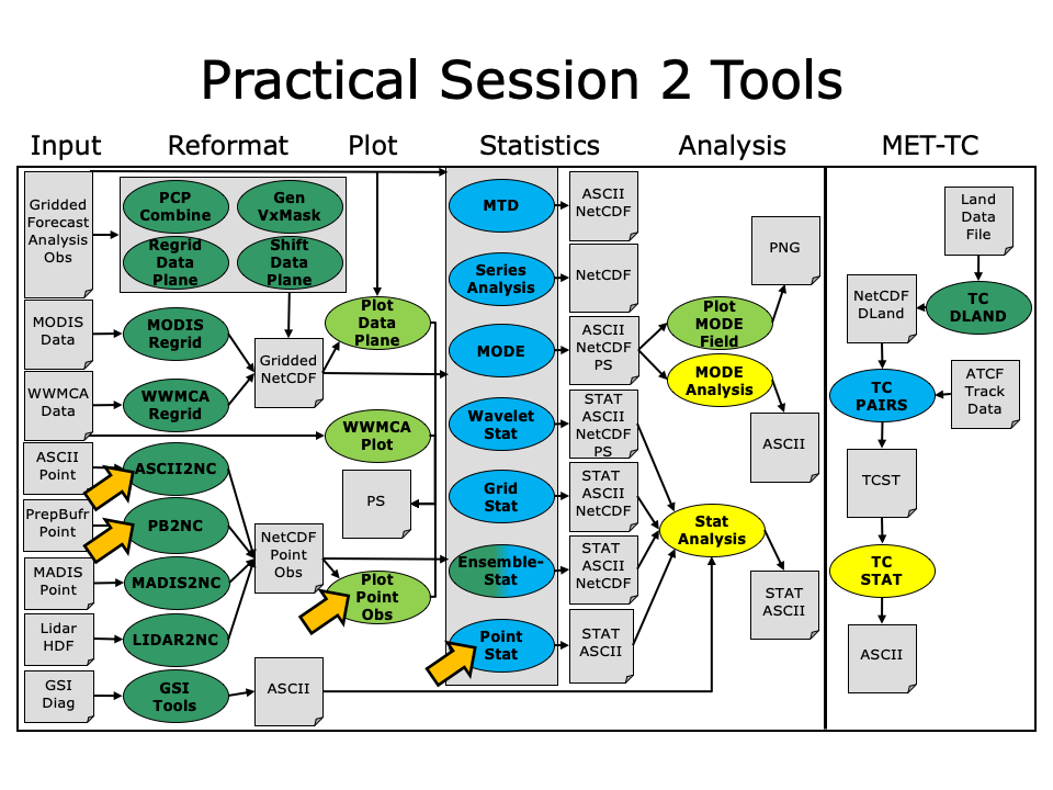
During this practical session, you will run the tools indicated below:
 You may navigate through this tutorial by following the links at the bottom of each page or by using the menu navigation.
Since you already set up your runtime enviroment in Session 1, you should be ready to go! To be sure, run through the following instructions to check that your environment is set correctly.
Prerequisites: Verify Environment is Set Correctly
Before running these instructions, you will need to ensure that you have a few environment variables set up correctly. If they are not set correctly, these instructions will not work properly.
- Check that you have METPLUS_TUTORIAL_DIR set correctly:
ls ${METPLUS_TUTORIAL_DIR}
If you don't see a path in your user directory output to the screen, set this environment variable in your user profile before continuing.
- Check that you have METPLUS_BUILD_BASE, MET_BUILD_BASE, and METPLUS_DATA set correctly:
echo ${MET_BUILD_BASE}
echo ${METPLUS_DATA}
ls ${METPLUS_BUILD_BASE}
ls ${MET_BUILD_BASE}
ls ${METPLUS_DATA}
If any of these variables are not set, please set them. They will be referenced throughout the tutorial.
MET_BUILD_BASE is the full path to the MET installation (/path/to/met-X.Y)
METPLUS_DATA is the location of the sample test data directory
- Check that you have loaded the MET module correctly:
You should see the usage statement for Point-Stat. The version number listed should correspond to the version listed in MET_BUILD_BASE. If it does not, you will need to either reload the met module, or add ${MET_BUILD_BASE}/bin to your PATH.
- Check that METPLUS_PARM_BASE was set correctly.
ls ${METPLUS_PARM_BASE}
If you don't see the full path to your METplus/parm directory under the tutorial directory, please set it. See the instructions in Session 1 for more information.
- Check that the correct version of master_metplus.py is in your PATH:
If you don't see the full path to script from the shared installation, please set it. It should look the same as the output from this command:
ls ${METPLUS_BUILD_BASE}/ush/master_metplus.py
See the instructions in Session 1 for more information.
You are now ready to move on to the next section.
MET Tool: PB2NC
MET Tool: PB2NC cindyhg Tue, 06/25/2019 - 09:25PB2NC Tool: General
PB2NC Functionality
The PB2NC tool is used to stratify (i.e. subset) the contents of an input PrepBufr point observation file and reformat it into NetCDF format for use by the Point-Stat or Ensemble-Stat tool. In this session, we will run PB2NC on a PrepBufr point observation file prior to running Point-Stat. Observations may be stratified by variable type, PrepBufr message type, station identifier, a masking region, elevation, report type, vertical level category, quality mark threshold, and level of PrepBufr processing. Stratification is controlled by a configuration file and discussed on the next page.
The PB2NC tool may be run on both PrepBufr and Bufr observation files. As of met-6.1, support for Bufr is limited to files containing embedded tables. Support for Bufr files using external tables will be added in a future release.
For more information about the PrepBufr format, visit:
http://www.emc.ncep.noaa.gov/mmb/data_processing/prepbufr.doc/document.htm
For information on where to download PrepBufr files, visit:
https://dtcenter.org/community-code/model-evaluation-tools-met/input-data
PB2NC Usage
View the usage statement for PB2NC by simply typing the following:
| Usage: pb2nc | ||
| prepbufr_file | input prepbufr path/filename | |
| netcdf_file | output netcdf path/filename | |
| config_file | configuration path/filename | |
| [-pbfile prepbufr_file] | additional input files | |
| [-valid_beg time] | Beginning of valid time window [YYYYMMDD_[HH[MMSS]]] | |
| [-valid_end time] | End of valid time window [YYYYMMDD_[HH[MMSS]]] | |
| [-nmsg n] | Number of PrepBufr messages to process | |
| [-index] | List available observation variables by message type (no output file) | |
| [-dump path] | Dump entire contents of PrepBufr file to directory | |
| [-log file] | Outputs log messages to the specified file | |
| [-v level] | Level of logging | |
| [-compression level] | NetCDF file compression |
At a minimum, the input prepbufr_file, the output netcdf_file, and the configuration config_file must be passed in on the command line. Also, you may use the -pbfile command line argument to run PB2NC using multiple input PrepBufr files, likely adjacent in time.
When running PB2NC on a new dataset, users are advised to run with the -index option to list the observation variables that are present in that file.
PB2NC Tool: Configure
PB2NC Tool: Configure cindyhg Tue, 06/25/2019 - 09:26PB2NC Tool: Configure
Start by making an output directory for PB2NC and changing directories:
cd ${METPLUS_TUTORIAL_DIR}/output/met_output/pb2nc
The behavior of PB2NC is controlled by the contents of the configuration file passed to it on the command line. The default PB2NC configuration may be found in the data/config/PB2NCConfig_default file. Prior to modifying the configuration file, users are advised to make a copy of the default:
Open up the PB2NCConfig_tutorial_run1 file for editing with your preferred text editor.
The configurable items for PB2NC are used to filter out the PrepBufr observations that should be retained or derived. You may find a complete description of the configurable items in section 4.1.2 of the MET User's Guide or in the configuration README file.
For this tutorial, edit the PB2NCConfig_tutorial_run1 file as follows:
- Set:
message_type = [ "ADPUPA", "ADPSFC" ];To retain only those 2 message types. Message types are described in:
http://www.emc.ncep.noaa.gov/mmb/data_processing/prepbufr.doc/table_1.htm - Set:
obs_window = {
beg = -30*60;
end = 30*60;
}So that only observations within 30 minutes of the file time will be retained.
- Set:
mask = {
grid = "G212";
poly = "";
}To retain only those observations residing within NCEP Grid 212, on which the forecast data resides.
- Set:
obs_bufr_var = [ "QOB", "TOB", "UOB", "VOB", "D_WIND", "D_RH" ];To retain observations for specific humidity, temperature, the u-component of wind, and the v-component of wind and to derive observation values for wind speed and relative humidity.
While we are request these observation variable names from the input file, the following corresponding strings will be written to the output file: SPFH, TMP, UGRD, VGRD, WIND, RH. This mapping of input PrepBufr variable names to output variable names is specified by the obs_prepbufr_map config file entry. This enables the new features in the current version of MET to be backward compatible with earlier versions.
Next, save the PB2NCConfig_tutorial_run1 file and exit the text editor.
PB2NC Tool: Run
PB2NC Tool: Run cindyhg Tue, 06/25/2019 - 09:27PB2NC Tool: Run
Next, run PB2NC on the command line using the following command:
${METPLUS_DATA}/met_test/data/sample_obs/prepbufr/ndas.t00z.prepbufr.tm12.20070401.nr \
tutorial_pb_run1.nc \
PB2NCConfig_tutorial_run1 \
-v 2
If this run fails due to runtime issues, please download a copy of the output file here and manually save it as tutorial_pb_run1.nc.
PB2NC is now filtering the observations from the PrepBufr file using the configuration settings we specified and writing the output to the NetCDF file name we chose. This should take a few minutes to run. As it runs, you should see several status messages printed to the screen to indicate progress. You may use the -v command line option to turn off (-v 0) or change the amount of log information printed to the screen.
Inspect the PB2NC status messages and note that 69833 PrepBufr messages were filtered down to 8394 messages which produced 52491 actual and derived observations. If you'd like to filter down the observations further, you may want to narrow the time window or modify other filtering criteria. We will do that after inspecting the resultant NetCDF file.
PB2NC Tool: Output
PB2NC Tool: Output cindyhg Tue, 06/25/2019 - 09:29PB2NC Tool: Output
When PB2NC is finished, you may view the output NetCDF file it wrote using the ncdump utility. Run the following command to view the header of the NetCDF output file:
In the NetCDF header, you'll see that the file contains nine dimensions and nine variables. The obs_arr variable contains the actual observation values. The obs_qty variable contains the corresponding quality flags. The four header variables (hdr_typ, hdr_sid, hdr_vld, hdr_arr) contain information about the observing locations.
The obs_var, obs_unit, and obs_desc variables describe the observation variables contained in the output. The second entry of the obs_arr variable (i.e. var_id) lists the index into these array for each observation. For example, for observations of temperature, you'd see TMP in obs_var, KELVIN in obs_unit, and TEMPERATURE OBSERVATION in obs_desc. For observations of temperature in obs_arr, the second entry (var_id) would list the index of that temperature information.
Inspect the output of ncdump before continuing.
Plot-Point-Obs
The plot_point_obs tool plots the location of these NetCDF point observations. Just like plot_data_plane is useful to visualize gridded data, run plot_point_obs to make sure you have point observations where you expect. Run the following command:
tutorial_pb_run1.nc \
tutorial_pb_run1.ps
Display the output PostScript file by running the following command:
Each red dot in the plot represents the location of at least one observation value. The plot_point_obs tool has additional command line options for filtering which observations get plotted and the area to be plotted. View its usage statement by running the following command:
By default, the points are plotted on the full globe. Next, try rerunning plot_point_obs using the -data_file option to specify the grid over which the points should be plotted:
tutorial_pb_run1.nc \
tutorial_pb_run1_zoom.ps \
-data_file ${METPLUS_DATA}/met_test/data/sample_fcst/2007033000/nam.t00z.awip1236.tm00.20070330.grb
MET extracts the grid information from the first record of that GRIB file and plots the points on that domain. Display the output PostScript file by running the following command:
The plot_data_plane tool can be run on the NetCDF output of any of the MET point observation pre-processing tools (pb2nc, ascii2nc, madis2nc, and lidar2nc).
PB2NC Tool: Reconfigure and Rerun
PB2NC Tool: Reconfigure and Rerun cindyhg Tue, 06/25/2019 - 09:31PB2NC Tool: Reconfigure and Rerun
Now we'll rerun PB2NC, but this time we'll tighten the observation acceptance criteria. Start by making a copy of the configuration file we just used:
Open up the PB2NCConfig_tutorial_run2 file and edit it as follows:
- Set:
message_type = [];To retain all message types.
- Set:
obs_window = {
beg = -25*60;
end = 25*60;
}So that only observations 25 minutes before and 25 minutes after the top of the hour are retained.
- Set:
quality_mark_thresh = 1;To retain only the observations marked "Good" by the NCEP quality control system.
Next, run PB2NC again but change the output name using the following command:
${METPLUS_DATA}/met_test/data/sample_obs/prepbufr/ndas.t00z.prepbufr.tm12.20070401.nr \
tutorial_pb_run2.nc \
PB2NCConfig_tutorial_run2 \
-v 2
If this run fails due to runtime issues, please download a copy of the output file here and manually save it as tutorial_pb_run2.nc.
Inspect the PB2NC status messages and note that 4000 observations were retained rather than 52491 in the previous example. The majority of the observations were rejected because their valid time no longer fell inside the tighter obs_window setting.
When configuring PB2NC for your own projects, you should err on the side of keeping more data rather than less. As you'll see, the grid-to-point verification tools (Point-Stat and Ensemble-Stat) allow you to further refine which point observations are actually used in the verification. However, keeping a lot of point observations that you'll never actually use will make the data files larger and slightly slow down the verification. For example, if you're using a Global Data Assimilation (GDAS) PREPBUFR file to verify a model over Europe, it would make sense to only keep those point observations that fall within your model domain.
MET Tool: ASCII2NC
MET Tool: ASCII2NC cindyhg Tue, 06/25/2019 - 09:32ASCII2NC Tool: General
ASCII2NC Functionality
The ASCII2NC tool reformats ASCII point observations into the intermediate NetCDF format that Point-Stat and Ensemble-Stat read. ASCII2NC simply reformats the data and does much less filtering of the observations than PB2NC does. ASCII2NC supports a simple 11-column format, described below, the Little-R format often used in data assimilation, surface radiation (SURFRAD) data, Western Wind and Solar Integration Studay (WWSIS) data, and AErosol RObotic NEtwork (Aeronet) data. Future version of MET may be enhanced to support additional commonly used ASCII point observation formats based on community input.
MET Point Observation Format
The MET point observation format consists of one observation value per line. Each input observation line should consist of the following 11 columns of data:
- Message_Type
- Station_ID
- Valid_Time in YYYYMMDD_HHMMSS format
- Lat in degrees North
- Lon in degrees East
- Elevation in meters above sea level
- Variable_Name for this observation (or GRIB_Code for backward compatibility)
- Level as the pressure level in hPa or accumulation interval in hours
- Height in meters above sea level or above ground level
- QC_String quality control string
- Observation_Value
It is the user's responsibility to get their ASCII point observations into this format.
ASCII2NC Usage
View the usage statement for ASCII2NC by simply typing the following:
| Usage: ascii2nc | ||
| ascii_file1 [...] | One or more input ASCII path/filename | |
| netcdf_file | Output NetCDF path/filename | |
| [-format ASCII_format] | Set to met_point, little_r, surfrad, wwsis, or aeronet | |
| [-config file] | Configuration file to specify how observation data should be summarized | |
| [-mask_grid string] | Named grid or a gridded data file for filtering point observations spatially | |
| [-mask_poly file] | Polyline masking file for filtering point observations spatially | |
| [-mask_sid file|list] | Specific station ID's to be used in an ASCII file or comma-separted list | |
| [-log file] | Outputs log messages to the specified file | |
| [-v level] | Level of logging | |
| [-compress level] | NetCDF compression level |
At a minimum, the input ascii_file and the output netcdf_file must be passed on the command line. ASCII2NC interrogates the data to determine it's format, but the user may explicitly set it using the -format command line option. The -mask_grid, -mask_poly, and -mask_sid options can be used to filter observations spatially.
ASCII2NC Tool: Run
ASCII2NC Tool: Run cindyhg Tue, 06/25/2019 - 09:33ASCII2NC Tool: Run
Start by making an output directory for ASCII2NC and changing directories:
cd ${METPLUS_TUTORIAL_DIR}/output/met_output/ascii2nc
Since ASCII2NC performs a simple reformatting step, typically no configuration file is needed. However, when processing high-frequency (1 or 3-minute) SURFRAD data, a configuration file may be used to define a time window and summary metric for each station. For example, you might compute the average observation value +/- 15 minutes at the top of each hour for each station. In this example, we will not use a configuration file.
The sample ASCII observations in the MET tarball are still identified by GRIB code rather than the newer variable name option. Dump that file and notice that the GRIB codes in the seventh column could be replaced by corresponding variable names. For example, 52 corresponds to RH:
Run ASCII2NC on the command line using the following command:
${METPLUS_DATA}/met_test/data/sample_obs/ascii/sample_ascii_obs.txt \
tutorial_ascii.nc \
-v 2
ASCII2NC should perform this reformatting step very quickly since the sample file only contains data for 5 stations.
ASCII2NC Tool: Output
ASCII2NC Tool: Output cindyhg Tue, 06/25/2019 - 09:37ASCII2NC Tool: Output
When ASCII2NC is finished, you may view the output NetCDF file it wrote using the ncdump utility. Run the following command to view the header of the NetCDF output file:
The NetCDF header should look nearly identical to the output of the NetCDF output of PB2NC. You can see the list of stations for which we have data by inspecting the hdr_sid_table variable:
Feel free to inspect the contents of the other variables as well.
This ASCII data only contains observations at a few locations. Use the plot_point_obs to plot the locations, increasing the level of verbosity to 3 to see more detail:
tutorial_ascii.nc \
tutorial_ascii.ps \
-data_file ${METPLUS_DATA}/met_test/data/sample_fcst/2007033000/nam.t00z.awip1236.tm00.20070330.grb \
-v 3
Next, we'll use the NetCDF output of PB2NC and ASCII2NC to perform Grid-to-Point verification using the Point-Stat tool.
MET Tool: Point-Stat
MET Tool: Point-Stat cindyhg Tue, 06/25/2019 - 09:38Point-Stat Tool: General
Point-Stat Functionality
The Point-Stat tool provides verification statistics for comparing gridded forecasts to observation points, as opposed to gridded analyses like Grid-Stat. The Point-Stat tool matches gridded forecasts to point observation locations using one or more configurable interpolation methods. The tool then computes a configurable set of verification statistics for these matched pairs. Continuous statistics are computed over the raw matched pair values. Categorical statistics are generally calculated by applying a threshold to the forecast and observation values. Confidence intervals, which represent a measure of uncertainty, are computed for all of the verification statistics.
Point-Stat Usage
View the usage statement for Point-Stat by simply typing the following:
| Usage: point_stat | ||
| fcst_file | Input gridded file path/name | |
| obs_file | Input NetCDF observation file path/name | |
| config_file | Configuration file | |
| [-point_obs file] | Additional NetCDF observation files to be used (optional) | |
| [-obs_valid_beg time] | Sets the beginning of the matching time window in YYYYMMDD[_HH[MMSS]] format (optional) | |
| [-obs_valid_end time] | Sets the end of the matching time window in YYYYMMDD[_HH[MMSS]] format (optional) | |
| [-outdir path] | Overrides the default output directory (optional) | |
| [-log file] | Outputs log messages to the specified file (optional) | |
| [-v level] | Level of logging (optional) |
At a minimum, the input gridded fcst_file, the input NetCDF obs_file (output of PB2NC, ASCII2NC, MADIS2NC, and LIDAR2NC, last two not covered in these exercises), and the configuration config_file must be passed in on the command line. You may use the -point_obs command line argument to specify additional NetCDF observation files to be used.
Point-Stat Tool: Configure
Point-Stat Tool: Configure cindyhg Tue, 06/25/2019 - 09:40Point-Stat Tool: Configure
Start by making an output directory for Point-Stat and changing directories:
cd ${METPLUS_TUTORIAL_DIR}/output/met_output/point_stat
The behavior of Point-Stat is controlled by the contents of the configuration file passed to it on the command line. The default Point-Stat configuration file may be found in the data/config/PointStatConfig_default file.
The configurable items for Point-Stat are used to specify how the verification is to be performed. The configurable items include specifications for the following:
- The forecast fields to be verified at the specified vertical levels.
- The type of point observations to be matched to the forecasts.
- The threshold values to be applied.
- The areas over which to aggregate statistics - as predefined grids, lat/lon polylines, or individual stations.
- The confidence interval methods to be used.
- The interpolation methods to be used.
- The types of verification methods to be used.
Let's customize the configuration file. First, make a copy of the default:
Next, open up the PointStatConfig_tutorial_run1 file for editing and modify it as follows:
- Set:
fcst = {
wind_thresh = [ NA ];
message_type = [ "ADPUPA" ];
field = [
{
name = "TMP";
level = [ "P850-1050", "P500-850" ];
cat_thresh = [ <=273, >273 ];
}
];
}
obs = fcst; - To verify temperature over two different pressure ranges against ADPUPA observations using the thresholds specified.
- Set:
ci_alpha = [ 0.05, 0.10 ];To compute confidence intervals using both a 5% and a 10% level of certainty.
- Set:
output_flag = {
fho = BOTH;
ctc = BOTH;
cts = STAT;
mctc = NONE;
mcts = NONE;
cnt = BOTH;
sl1l2 = STAT;
sal1l2 = NONE;
vl1l2 = NONE;
val1l2 = NONE;
pct = NONE;
pstd = NONE;
pjc = NONE;
prc = NONE;
ecnt = NONE;
eclv = BOTH;
mpr = BOTH;
}To indicate that the forecast-hit-observation (FHO) counts, contingency table counts (CTC), contingency table statistics (CTS), continuous statistics (CNT), partial sums (SL1L2), economic cost/loss value (ECLV), and the matched pair data (MPR) line types should be output. Setting SL1L2 and CTS to STAT causes those lines to only be written to the output .stat file, while setting others to BOTH causes them to be written to both the .stat file and the optional LINE_TYPE.txt file.
- Set:
output_prefix = "run1";To customize the output file names for this run.
Note in this configuration file that in the mask dictionary, the grid entry is set to FULL. This instructs Point-Stat to compute statistics over the entire input model domain. Setting grid to FULL has this special meaning.
Next, save the PointStatConfig_tutorial_run1 file and exit the text editor.
Point-Stat Tool: Run
Point-Stat Tool: Run cindyhg Tue, 06/25/2019 - 09:41Point-Stat Tool: Run
Next, run Point-Stat to compare a GRIB forecast to the NetCDF point observation output of the ASCII2NC tool. Run the following command line:
${METPLUS_DATA}/met_test/data/sample_fcst/2007033000/nam.t00z.awip1236.tm00.20070330.grb \
../ascii2nc/tutorial_ascii.nc \
PointStatConfig_tutorial_run1 \
-outdir . \
-v 2
Point-Stat is now performing the verification tasks we requested in the configuration file. It should take less than a minute to run. You should see several status messages printed to the screen to indicate progress.
Now try rerunning the command listed above, but increase the verbosity level to 3 (-v 3). Notice the more detailed information about which observations were used for each verification task. If you run Point-Stat and get fewer matched pairs than you expected, try using the -v 3 option to see why the observations were rejected.
Users often write MET-Help to ask why they got zero matched pairs from Point-Stat. The first step is always rerunning Point-Stat using verbosity level 3 or higher to list the counts of reasons for why observations were not used!
Point-Stat Tool: Output
Point-Stat Tool: Output cindyhg Tue, 06/25/2019 - 09:42Point-Stat Tool: Output
The output of Point-Stat is one or more ASCII files containing statistics summarizing the verification performed. Since we wrote output to the current directory, it should now contain 6 ASCII files that begin with the point_stat_ prefix, one each for the FHO, CTC, CNT, ECLV, and MPR types, and a sixth for the STAT file. The STAT file contains all of the output statistics while the other ASCII files contain the exact same data organized by line type.
Since the lines of data in these ASCII files are so long, we strongly recommend configuring your text editor to NOT use dynamic word wrapping. The files will be much easier to read that way:
- In the kwrite editor, select Settings->Configure Editor, de-select Dynamic Word Wrap and click OK.
- In the vi editor, type the command :set nowrap. To set this as the default behavior, run the following command:
echo "set nowrap" >> ~/.exrc
Open up the point_stat_run1_360000L_20070331_120000V_ctc.txt CTC file using the text editor of your choice and note the following:
- This is a simple ASCII file consisting of several rows of data.
- Each row contains data for a single verification task.
- The FCST_LEAD, FCST_VALID_BEG, and FCST_VALID_END columns indicate the timing information of the forecast field.
- The OBS_LEAD, OBS_VALID_BEG, and OBS_VALID_END columns indicate the timing information of the observation field.
- The FCST_VAR, FCST_LEV, OBS_VAR, and OBS_LEV columns indicate the two parts of the forecast and observation fields set in the configure file.
- The OBTYPE column indicates the PrepBufr message type used for this verification task.
- The VX_MASK column indicates the masking region over which the statistics were accumulated.
- The INTERP_MTHD and INTERP_PNTS columns indicate the method used to interpolate the forecast data to the observation location.
- The FCST_THRESH and OBS_THRESH columns indicate the thresholds applied to FCST_VAR and OBS_VAR.
- The COV_THRESH column is not applicable here and will always have NA when using point_stat.
- The ALPHA column indicates the alpha used for confidence intervals.
- The LINE_TYPE column indicates that these are CTC contingency table count lines.
- The remaining columns contain the counts for the contingency table computed by applying the threshold to the forecast/observation matched pairs. The FY_OY (forecast: yes, observation: yes), FY_ON (forecast: yes, observation: no), FN_OY (forecast: no, observation: yes), and FN_ON (forecast: no, observation: no) columns indicate those counts.
Next, answer the following questions about this contingency table output:
- What do you notice about the structure of the contingency table counts with respect to the two thresholds used? Does this make sense?
- Does the model appear to resolve relatively cold surface temperatures?
- Based on these observations, are temperatures >273 relatively rare or common in the P850-500 range? How can this affect the ability to get a good score using contingency table statistics? What about temperatures <=273 at the surface?
Close that file, open up the point_stat_run1_360000L_20070331_120000V_cnt.txt CNT file, and note the following:
- The columns prior to LINE_TYPE contain the same data as the previous file we viewed.
- The LINE_TYPE column indicates that these are CNT continuous lines.
- The remaining columns contain continuous statistics derived from the raw forecast/observation pairs. See section 4.3.3 of the MET User's Guide for a thorough description of the output.
- Again, confidence intervals are given for each of these statistics as described above.
Next, answer the following questions about these continuous statistics:
- What conclusions can you draw about the model's performance at each level using continuous statistics? Justify your answer. Did you use a single metric in your evaluation? Why or why not?
- Comparing the first line with an alpha value of 0.05 to the second line with an alpha value of 0.10, how does the level of confidence change the upper and lower bounds of the confidence intervals (CIs)?
- Similarily, comparing the first line with few numbers of matched pairs in the TOTAL column to the third line with more, how does the sample size affect how you interpret your results?
Close that file, open up the point_stat_run1_360000L_20070331_120000V_fho.txt FHO file, and note the following:
- The columns prior to LINE_TYPE contain the same data as the previous file we viewed.
- The LINE_TYPE column indicates that these are FHO forecast-hit-observation rate lines.
- The remaining columns are similar to the contingency table output and contain the total number of matched pairs, the forecast rate, the hit rate, and observation rate.
- The forecast, hit, and observation rates should back up your answer to the third question about the contingency table output.
Close that file, open up the point_stat_run1_360000L_20070331_120000V_mpr.txt MPR file, and note the following:
- The columns prior to LINE_TYPE contain the same data as the previous file we viewed.
- The LINE_TYPE column indicates that these are MPR matched pair lines.
- The remaining columns are similar to the contingency table output and contain the total number of matched pairs, the matched pair index, the latitude, longitude, and elevation of the observation, the forecasted value, the observed value, and the climatologic value (if applicable).
- There is a lot of data here and it is recommended that the MPR line_type is used only to verify the tool is working properly.
Point-Stat Tool: Reconfigure
Point-Stat Tool: Reconfigure cindyhg Tue, 06/25/2019 - 09:44Point-Stat Tool: Reconfigure
Now we'll reconfigure and rerun Point-Stat. Start by making a copy of the configuration file we just used:
This time, we'll use two dictionary entries to specify the forecast field in order to set different thresholds for each vertical level. Point-Stat may be configured to verify as many or as few model variables and vertical levels as you desire. Edit the PointStatConfig_tutorial_run2 file as follows:
- Set:
fcst = {
wind_thresh = [ NA ];
message_type = [ "ADPUPA", "ADPSFC" ];
field = [
{
name = "TMP";
level = [ "Z2" ];
cat_thresh = [ >273, >278, >283, >288 ];
},
{
name = "TMP";
level = [ "P750-850" ];
cat_thresh = [ >278 ];
}
];
}
obs = fcst;To verify 2-meter temperature and temperature fields between 750hPa and 850hPa, using the thresholds specified, and by comparing against the two message types.
- Set:
mask = {
grid = [ "G212" ];
poly = [ "MET_BASE/poly/EAST.poly",
"MET_BASE/poly/WEST.poly" ];
sid = [];
llpnt = [];
}To compute statistics over the NCEP Grid 212 region and over the Eastern and Western United States, as defined by the polylines specified.
- Set:
interp = {
vld_thresh = 1.0;
type = [
{
method = NEAREST;
width = 1;
},
{
method = DW_MEAN;
width = 5;
}
];
}To indicate that the forecast values should be interpolated to the observation locations using the nearest neighbor method and by computing a distance-weighted average of the forecast values over the 5 by 5 box surrounding the observation location.
- Set:
output_flag = {
fho = BOTH;
ctc = BOTH;
cts = BOTH;
mctc = NONE;
mcts = NONE;
cnt = BOTH;
sl1l2 = BOTH;
sal1l2 = NONE;
vl1l2 = NONE;
val1l2 = NONE;
pct = NONE;
pstd = NONE;
pjc = NONE;
prc = NONE;
ecnt = NONE;
eclv = BOTH;
mpr = BOTH;
}To switch the SL1L2 and CTS output to BOTH and generate the optional ASCII output files for them.
- Set:
output_prefix = "run2";To customize the output file names for this run.
Let's look at our configuration selections and figure out the number of verification tasks Point-Stat will perform:
- 2 fields: TMP/Z2 and TMP/P750-850
- 2 observing message types: ADPUPA and ADPSFC
- 3 masking regions: G212, EAST.poly, and WEST.poly
- 2 interpolations: UW_MEAN width 1 (nearest-neighbor) and DW_MEAN width 5
Multiplying 2 * 2 * 3 * 2 = 24. So in this example, Point-Stat will accumulate matched forecast/observation pairs into 24 groups. However, some of these groups will result in 0 matched pairs being found. To each non-zero group, the specified threshold(s) will be applied to compute contingency tables.
Can you diagnose why some of these verification tasks resulted in zero matched pairs? (Hint: Reread the tip two pages back!)
Point-Stat Tool: Rerun
Point-Stat Tool: Rerun cindyhg Tue, 06/25/2019 - 09:45Point-Stat Tool: Rerun
Next, run Point-Stat to compare a GRIB forecast to the NetCDF point observation output of the PB2NC tool, as opposed to the much smaller ASCII2NC output we used in the first run. Run the following command line:
${METPLUS_DATA}/met_test/data/sample_fcst/2007033000/nam.t00z.awip1236.tm00.20070330.grb \
../pb2nc/tutorial_pb_run1.nc \
PointStatConfig_tutorial_run2 \
-outdir . \
-v 2
Point-Stat is now performing the verification tasks we requested in the configuration file. It should take a minute or two to run. You should see several status messages printed to the screen to indicate progress. Note the number of matched pairs found for each verification task, some of which are 0.
Plot-Data-Plane Tool
In this step, we have verified 2-meter temperature. The Plot-Data-Plane tool within MET provides a way to visualize the gridded data fields that MET can read. Run this utility to plot the 2-meter temperature field:
${METPLUS_DATA}/met_test/data/sample_fcst/2007033000/nam.t00z.awip1236.tm00.20070330.grb \
nam.t00z.awip1236.tm00.20070330_TMPZ2.ps \
'name="TMP"; level="Z2";'
Plot-Data-Plane requires an input gridded data file, an output postscript image file name, and a configuration string defining which 2-D field is to be plotted. View the output by running:
View the usage for Plot-Data-Plane by running it with no arguments or using the --help option:
Now rerun this Plot-Data-Plane command but...
- Set the title to 2-m Temperature.
- Set the plotting range as 250 to 305.
- Use the color table named ${MET_BUILD_BASE}/share/met/colortables/NCL_colortables/wgne15.ctable
Next, we'll take a look at the Point-Stat output we just generated.
See the usage statement for all MET tools using the --help command line option or with no options at all.
Point-Stat Tool: Output
Point-Stat Tool: Output cindyhg Tue, 06/25/2019 - 09:46Point-Stat Tool: Output
The format for the CTC, CTS, and CNT line types are the same. However, the numbers will be different as we used a different set of observations for the verification.
Open up the point_stat_run2_360000L_20070331_120000V_cts.txt CTS file, and note the following:
- The columns prior to LINE_TYPE contain header information.
- The LINE_TYPE column indicates that these are CTS lines.
- The remaining columns contain statistics derived from the threshold contingency table counts. See section 7.3.3 of the MET User's Guide for a thorough description of the output.
- Confidence intervals are given for each of these statistics, computed using either one or two methods. The columns ending in _NCL(normal confidence lower) and _NCU (normal confidence upper) give lower and upper confidence limits computed using assumptions of normality. The columns ending in _BCL (bootstrap confidence lower) and _BCU (bootstrap confidence upper) give lower and upper confidence limits computed using bootstrapping.
Close that file, open up the point_stat_run2_360000L_20070331_120000V_sl1l2.txt SL1L2 partial sums file, and note the following:
- The columns prior to LINE_TYPE contain header information.
- The LINE_TYPE column indicates these are SL1L2 partial sums lines.
Lastly, the point_stat_run2_360000L_20070331_120000V.stat file contains all of the same data we just viewed but in a single file. The Stat-Analysis tool, which we'll use later in this tutorial, searches for the .stat output files by default but can also read the .txt output files.
Use Case: Grid-to-Obs
Use Case: Grid-to-Obs cindyhg Tue, 06/25/2019 - 09:48METplus Use Case: Grid to Obs Upper Air
The Grid to Obs Upper Air use case utilizes the MET PB2NC and Point-Stat tools.
The default statistics created by this use case only dump the partial sums, so we will be also modifying the MET configuration file to add the continuous statistics to the output.
There is a little more setup in this use case, which will be instructive and demonstrate the basic structure, flexibility and setup of METplus configuration.
Optional, Refer to the MET Users Guide for a description of the MET tools used in this use case.
Optional, Refer to the METplus Users Guide for a reference to METplus variables used in this use case.
- Create Custom Configuration File
Define a unique directory under output that you will use for this use case. Create a configuration file to override OUTPUT_BASE to that directory.
Set OUTPUT_BASE to contain a subdirectory specific to the Grid to Obs use case. Make sure to put it under the [dir] section.
OUTPUT_BASE = {ENV[METPLUS_TUTORIAL_DIR]}/output/grid_to_obs
Using this custom configuration file and the Grid to Obs use case configuration files that are distributed with METplus, you should be able to run the use case using the sample input data set without any other changes.
- Copy NetCDF data (output from PB2NC) to output directory
Since pb2nc takes 20 minutes to run on the sample data for this use case, we have pregenerated the netcdf output and will be copying this data to the OUTPUT_BASE directory.
cp -r ${METPLUS_DATA}/grid_to_obs/netcdf/* ${METPLUS_TUTORIAL_DIR}/output/grid_to_obs/
- Change the METplus PROCESS_LIST configuration variable for this use case to only run PointStat.
Review the use case configuration file and find the PROCESS_LIST value. Take not of how it is formatted.
Edit g2o.output.conf to override the PROCESS_LIST. PUT IT IN THE [config] SECTION!
PROCESS_LIST = PointStat
NOTE : PROCESS_LIST defines the processes that will be run for the use case.
- Review the settings in the Upper Air configuration file:
- Run the Grid to Obs Upper Air use case:
- Review the output files:
The following is the statistical ouput and files are generated from the command:
- point_stat_000000L_20170601_000000V.stat
- point_stat_000000L_20170602_000000V.stat
- point_stat_000000L_20170603_000000V.stat
METplus Use Case: Grid to Obs CONUS Surface
METplus Use Case: Grid to Obs CONUS Surface cindyhg Tue, 06/25/2019 - 09:53METplus Use Case: Grid to Obs CONUS Surface
The Grid to Obs CONUS Surface use case utilizes the MET PB2NC and Point-Stat tools.
The default statistics created by this use case only dump the partial sums, so we will be also modifying the MET configuration file to add the continuous statistics to the output.
There is a little more setup in this use case, which will be instructive and demonstrate the basic structure, flexibility and setup of METplus configuration.
Optional, Refer to the MET Users Guide for a description of the MET tools used in this use case.
Optional, Refer to the A-Z Config Glossary section of the METplus Users Guide for a reference to METplus variables used in this use case.
- Create Custom Configuration File
Define a unique directory under output that you will use for this use case. Create a configuration file to override OUTPUT_BASE to that directory.
Set OUTPUT_BASE to contain a subdirectory specific to the Grid to Obs use case. Make sure to put it under the [dir] section.
OUTPUT_BASE = {ENV[METPLUS_TUTORIAL_DIR]}/output/grid_to_obs_cs
Using this custom configuration file and the Grid to Obs use case configuration files that are distributed with METplus, you should be able to run the use case using the sample input data set without any other changes.
- Copy NetCDF data (output from PB2NC) to output directory
Since pb2nc takes 20 minutes to run on the sample data for this use case, we have pregenerated the netcdf output and will be copying this data to the OUTPUT_BASE directory.
cp -r ${METPLUS_DATA}/grid_to_obs/netcdf/* ${METPLUS_TUTORIAL_DIR}/output/grid_to_obs_cs/
- Change the METplus PROCESS_LIST configuration variable for this use case to only run PointStat.
Review the use case configuration file and find the PROCESS_LIST value. Take note of how it is formatted.
Edit g2o.output.conf to override the PROCESS_LIST. PUT IT IN THE [config] SECTION!
PROCESS_LIST = PointStat
NOTE : PROCESS_LIST defines the processes that will be run for the use case.
- Review the setting in the CONUS Surface configuration file:
- Run the Grid to Obs CONUS Surface use case:
You should see some ERROR messages output to the screen. The observation file for each run time could not be found.
- Debug Errors
Review the log file and read the ERROR messages.
Look in the directory that was searched to see what is in there. Copy the path output to the screen and list the contents.
You should see the following files
- prepbufr.nam.20170601.t00z.tm00.nc
- prepbufr.nam.20170602.t00z.tm00.nc
- prepbufr.nam.20170603.t00z.tm00.nc
Recall the ERROR message and the template that is being used to search for data:
The template we are using to find data does not match the actual data. The current template setting expects the following files:
- 20170601/nam.2017060100.nc
- 20170602/nam.2017060200.nc
- 20170603/nam.2017060300.nc
- Override the filename template for observation input to PointStat with the correct template.
Add it to g2o.cs.conf
OBS_POINT_STAT_INPUT_TEMPLATE = prepbufr.nam.{valid?fmt=%Y%m%d}.t{valid?fmt=%H}z.tm00.nc
- Rerun the Grid to Obs CONUS Surface use case:
If you set the template correctly, it should take a few minutes to run.
- Review the output files:
The following is the statistical ouput and files are generated from the command:
- point_stat_000000L_20170601_000000V.stat
- point_stat_000000L_20170602_000000V.stat
- point_stat_000000L_20170603_000000V.stat
Additional Exercises
Additional Exercises cindyhg Tue, 06/25/2019 - 09:55End of Practical Session 2
Congratulations! You have completed Session 2!
If you have extra time, you may want to try this additional METplus exercise.
EXERCISE 2.1: Rerun Point-Stat - Rerun Point-Stat to produce additional continuous statistics file types.
Instructions: Modify the METplus MET configuration file for Upper Air to write Continuous statistics (cnt) and the Vector Continuous Statistics (vcnt) line types to both the stat file and its own file.
To do this, you will edit your PointStatConfig_upper_air METPlus MET configuration file as below.
... other entries ...
cnt = BOTH;
vcnt = BOTH;
Rerun master_metplus
Review the additional output files generated under
Session 3: Ensemble and PQPF
Session 3: Ensemble and PQPF admin Wed, 06/12/2019 - 16:58METplus Practical Session 3
During this practical session, you will run the tools indicated below:
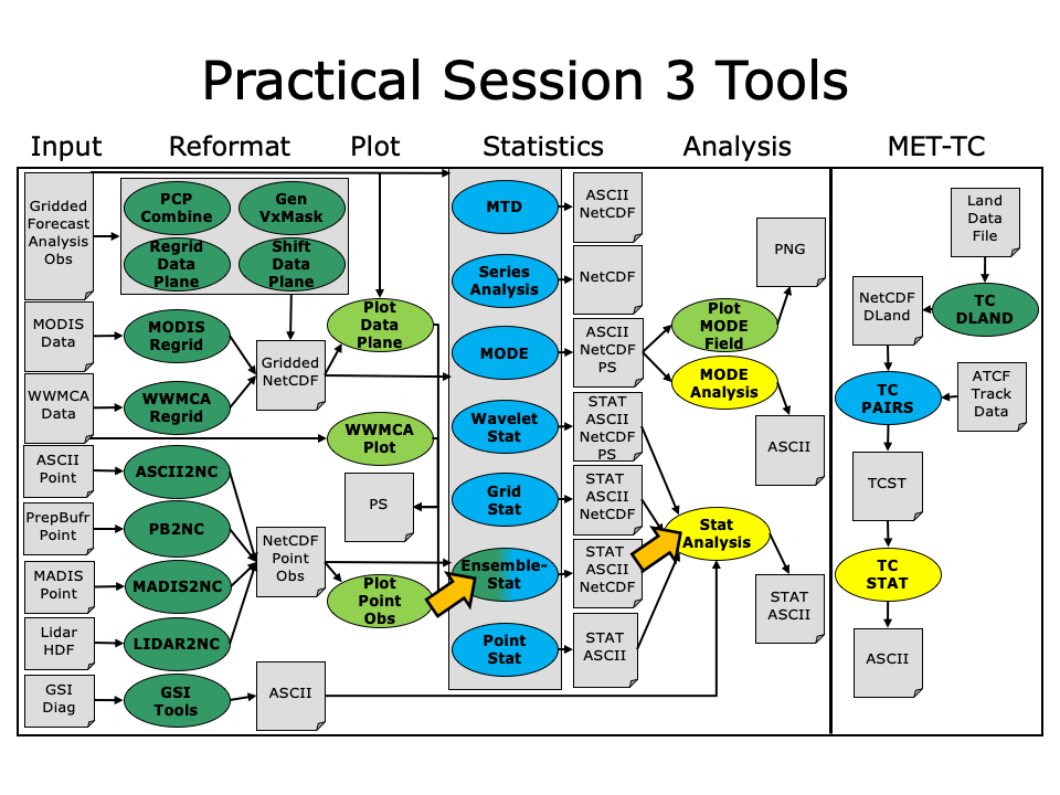
You may navigate through this tutorial by following the links at the bottom of each page or by using the menu navigation.
Since you already set up your runtime enviroment in Session 1, you should be ready to go! To be sure, run through the following instructions to check that your environment is set correctly.
Prerequisites: Verify Environment is Set Correctly
Before running these instructions, you will need to ensure that you have a few environment variables set up correctly. If they are not set correctly, these instructions will not work properly.
- Check that you have METPLUS_TUTORIAL_DIR set correctly:
ls ${METPLUS_TUTORIAL_DIR}
If you don't see a path in your user directory output to the screen, set this environment variable in your user profile before continuing.
- Check that you have METPLUS_BUILD_BASE, MET_BUILD_BASE, and METPLUS_DATA set correctly:
echo ${MET_BUILD_BASE}
echo ${METPLUS_DATA}
ls ${METPLUS_BUILD_BASE}
ls ${MET_BUILD_BASE}
ls ${METPLUS_DATA}
If any of these variables are not set, please set them. They will be referenced throughout the tutorial.
MET_BUILD_BASE is the full path to the MET installation (/path/to/met-X.Y)
METPLUS_DATA is the location of the sample test data directory
- Check that you have loaded the MET module correctly:
You should see the usage statement for Point-Stat. The version number listed should correspond to the version listed in MET_BUILD_BASE. If it does not, you will need to either reload the met module, or add ${MET_BUILD_BASE}/bin to your PATH.
- Check that METPLUS_PARM_BASE was set correctly.
ls ${METPLUS_PARM_BASE}
If you don't see the full path to your METplus/parm directory under the tutorial directory, please set it. See the instructions in Session 1 for more information.
- Check that the correct version of master_metplus.py is in your PATH:
If you don't see the full path to script from the shared installation, please set it. It should look the same as the output from this command:
ls ${METPLUS_BUILD_BASE}/ush/master_metplus.py
See the instructions in Session 1 for more information.
You are now ready to move on to the next section.
MET Tool: Ensemble-Stat
MET Tool: Ensemble-Stat cindyhg Tue, 06/25/2019 - 08:31Ensemble-Stat Tool: General
Ensemble-Stat Functionality
The Ensemble-Stat tool may be used to derive several summary fields, such as the ensemble mean, spread, and relative frequencies of events (i.e. similar to a probability). The summary fields produced by Ensemble-Stat may then be verified using the other MET statistics tools. Ensemble-Stat may also be used to verify the ensemble directly by comparing it to gridded and/or point observations. Statistics are then derived using those observations, such as rank histograms and the continuous ranked probability score.
Ensemble-Stat Usage
View the usage statement for Ensemble-Stat by simply typing the following:
At a minimum, the input gridded ensemble files and the configuration config_file must be passed in on the command line. You can specify the list of ensemble files to be used either as a count of the number of ensemble members followed by the file name for each (n_ens ens_fil e_1 ... ens_file_n) or as an ASCII file containing the names of the ensemble files to be used (ens_file_list). Choose whichever way is most convenient for you. The optional -grid_obs and -point_obs command line options may be used to specify gridde d and/or point observations to be used for computing rank histograms and other ensemble statistics.
As with the other MET statistics tools, all ensemble data and gridded verifying observations must be interpolated to a common grid prior to processing. This may be done using the automated regrid feature in the Ensemble-Stat configuration file or by running copygb and/or wgrib2 first.
Ensemble-Stat Tool: Configure
Ensemble-Stat Tool: Configure johnhg Thu, 07/25/2019 - 16:07Start by making an output directory for Ensemble-Stat and changing directories:
cd ${METPLUS_TUTORIAL_DIR}/output/met_output/ensemble_stat
The behavior of Ensemble-Stat is controlled by the contents of the configuration file passed to it on the command line. The default Ensemble-Stat configuration file may be found in the data/config/EnsembleStatConfig_default file. The configurations used by the test script may be found in the scripts/config/EnsembleStatConfig* files. Prior to modifying the configuration file, users are advised to make a copy of the default:
Open up the EnsembleStatConfig_tutorial file for editing with your preferred text editor.
The configurable items for Ensemble-Stat are broken out into two sections. The first section specifies how the ensemble should be processed to derive summary fields, such as the ensemble mean and spread. The second section specifies how the ensemble should be verified directly, such as the computation of rank histograms and spread/skill. The configurable items include specifications for the following:
- Section 1: Ensemble Processing (ens dictionary)
- The ensemble fields to be summarized at the specified vertical level or accumulation interval.
- The threshold values to be applied in computing ensemble relative frequencies (e.g. the percent of ensemble members exceeding some threshold at each point).
- Thresholds to specify how many of the ensemble members must actually be present with valid data.
- Section 2: Verification (fcst and obs dictionaries)
- The forecast and observation fields to be verified at the specified vertical level or accumulation interval.
- The matching time window for point observations.
- The type of point observations to be matched to the forecasts.
- The areas over which to aggregate statistics - as predefined grids or configurable lat/lon polylines.
- The interpolation or smoothing methods to be used.
You may find a complete description of the configurable items in section 9.3.2 of the MET User's Guide. Please take some time to review them.
For this tutorial, we'll configure Ensemble-Stat to summarize and verify 24-hour accumulated precipitation. While we'll run Ensemble-Stat on a single field, please note that it may be configured to operate on multiple fields. The ensemble we're verifying consists of 6 members defined over the west coast of the United States. Edit the EnsembleStatConfig_tutorial file as follows:
- In the ens dictionary, set
field = [
{
name = "APCP";
level = [ "A24" ];
cat_thresh = [ >0, >=5.0, >=10.0 ];
}
];To read 24-hour accumulated precipitation from the input GRIB files and compute ensemble relative frequencies for the thresolds listed.
- In the fcst dictionary, set
field = [
{
name = "APCP";
level = [ "A24" ];
}
];To also verify the 24-hour accumulated precipitation fields.
-
In the fcst dictionary, set:
message_type = [ "ADPSFC" ];To verify against surface observations.
- In the mask dictionary, set:
grid = [ "FULL" ];To accumulate statistics over the full model domain.
- In the mask dictionary, set
poly = [ "MET_BASE/poly/NWC.poly",
"MET_BASE/poly/SWC.poly" ];To also verify over the northwest coast (NWC) and southwest coast (SWC) subregions.
- Set:
output_flag = {
ecnt = BOTH;
rhist = BOTH;
phist = BOTH;
orank = BOTH;
ssvar = BOTH;
relp = BOTH;
}To compute continuous ensemble statistics (ECNT), ranked histogram (RHIST), probability integral transform histogram (PHIST), observation ranks (ORANK), spread-skill variance (SSVAR), and relative position (RELP).
Save and close this file.
Ensemble-Stat Tool: Run
Ensemble-Stat Tool: Run johnhg Thu, 07/25/2019 - 16:09Next, run Ensemble-Stat on the command line using the following command, using wildcards to list the 6 input ensemble member files:
6 ${METPLUS_DATA}/met_test/data/sample_fcst/2009123112/*gep*/d01_2009123112_02400.grib \
EnsembleStatConfig_tutorial \
-grid_obs ${METPLUS_DATA}/met_test/data/sample_obs/ST4/ST4.2010010112.24h \
-point_obs ${METPLUS_DATA}/met_test/out/ascii2nc/precip24_2010010112.nc \
-outdir . \
-v 2
 The command above uses the ASCII2NC output of that was generated by make test when MET was compiled.
Ensemble-Stat is now performing the tasks we requested in the configuration file. Note that we've passed the input ensemble data directly on the command line by specifying the number of ensemble members (6) followed by their names using wildcards. We've also specified one gridded StageIV analysis field (-grid_obs) and one file containing point rain gauge observations (-point_obs) to be used in computing rank histograms. This tool should run pretty quickly.
When Ensemble-Stat is finished, it will have created 9 output files in the current directory: 6 ASCII statistics files (.stat, _ecnt.txt, _rhist.txt, _phist.txt, _orank.txt, _ssvar.txt , and _relp.txt ) , a NetCDF ensemble file (_ens.nc), and a NetCDF matched pairs file (_orank.nc).
Ensemble-Stat Tool: Output
Ensemble-Stat Tool: Output johnhg Thu, 07/25/2019 - 16:11The _ens.nc output from Ensemble-Stat is a NetCDF file containing the derived ensemble fields, one or more ASCII files containing statistics summarizing the verification performed, and a NetCDF file containing the gridded matched pairs.
All of the line types are written to the file ending in .stat. The Ensemble-Stat tool currently writes six output line types, ECNT, RHIST, PHIST, RELP, SSVAR, and ORANK.
- The ECNT line type contains contains continuous ensemble statistics such as spread and skill. Ensemble-Stat uses assumed observation errors to compute both perturbed and unperturbed versions of these statistics. Statistics to which observation error have been applied can be found in columns which include the _OERR (for observation error) suffix.
- The RHIST line type contains counts for a ranked histogram. This ranks each observation value relative to ensemble member values. Ideally, observation values would fall equally across all available ranks, yiedling a flat rank histogram. In practice, ensembles are often under-(U shape) or over-(inverted U shape) dispersive. In the event of ties, ranks are randomly assigned.
- The PHIST line type contains counts for a probability integral transform histogram. This scales the observation ranks to a range of values between 0 and 1 and allows ensembles of different size to be compared. Similiary, when ensemble members drop out, RHIST lines cannot be aggregated together but PHIST lines can.
- The RELP line is the relative position, which indicates how often each ensemble member's value was closest to the observation's value. In the event of ties, credit is divided equally among the tied members.
- The ORANK line type is similar to the matched pair (MPR) output of Point-Stat. For each point observation value, one ORANK line is written out containing the observation value, it's rank, and the corresponding ensemble values for that point. When verifying against a griddedanalysis, the ranks can be written to the NetCDF output file.
- The SSVAR line contains binned spread/skill information. For each observation location, the ensemble variance is computed at that point. Those variance values are binned based on the ens_ssvar_bin_size configuration setting. The skill is deteremined by comparing the ensemble mean value to the observation value. One SSVAR line is written for each bin summarizing the all the observation/ensemble mean pairs that it contains.
The STAT file contains all the ASCII output while the _ecnt.txt, _rhist.txt, _phist.txt, _orank.txt, _ssvar.txt, and _relp.txtfiles contain the same data but sorted by line type. Since so much data can be written for the ORANK line type, we recommend disabling the output of the optional text file using the output_flag parameter in the configuration file.
Since the lines of data in these ASCII file are so long, we strongly recommend configuring your text editor to NOT use dynamic word wrapping. The files will be much easier to read that way.
Open up the ensemble_stat_20100101_120000V_rhist.txt RHIST file using the text editor of your choice and note the following:
- There are 6 lines in this output file resulting from using 3 verification regions in the VX_MASK column (FULL, NWC, and SWC) and two observations datasets in the OBTYPE column (ADPSFC point observations and gridded observations).
- Each line contains columns for the observations ranks (RANK_#) and a handful of ensemble statistics (CRPS, CRPSS, IGN, and SPREAD).
- There is output for 7 ranks - since we verified a 6-member ensemble, there are 7 possible ranks the observation values could attain.
Close this file, and open up the ensemble_stat_20100101_120000V_phist.txt PHIST file, and note the following:
- There are 5 lines in this output file resulting from using 3 verification regions (FULL, NWC, and SWC) and two observations datasets (ADPSFC point observations and gridded observations), where the ADPSFC point observations for the SWC region were all zeros for which the probability integral transform is not defined.
- Each line contains columns for the BIN_SIZE and counts for each bin. The bin size is set in the configuration file using the ens_phist_bin_size field. In this case, it was set to .05, therefore creating 20 bins (1/ens_phist_bin_size).
Close this file, and open up the ensemble_stat_20100101_120000V_orank.txt ORANK file, and note the following:
- This file contains 1866 lines, 1 line for each observation value falling inside each verification region (VX_MASK).
- Each line contains 44 columns... header information, the observation location and value, it's rank, and the 6 values for the ensemble members at that point.
- When there are ties, Ensemble-Stat randomly assigns a rank from all the possible choices. This can be seen in the SWC masking region where all of the observed values are 0 and the ensemble forecasts are 0 as well. Ensemble-Stat randomly assigns a rank between 1 and 7.
Close this file, and use the ncview utility to view the NetCDF ensemble fields file:
This file contains variables for the following:
- Ensemble Mean
- Ensemble Standard Deviation
- Ensemble Mean minus 1 Standard Deviation
- Ensemble Mean plus 1 Standard Deviation
- Ensemble Minimum
- Ensemble Maximum
- Ensemble Range
- Ensemble Valid Data Count
- Ensemble Relative Frequency (for 3 thresholds)
The output of any of these summary fields may be disabled using the output_flag parameter in the configuration file.
Use the ncview utility to view the NetCDF gridded observation rank file:
This file is only created when you've verified using gridded observations and have requested its output using the output_flagparameter in the configuration file. Click through the variables in this file. Note that for each of the three verification areas (FULL, NWC, and SWC) this file contains 4 variables:
- The gridded observation value
- The observation rank
- The probability integral transform
- The ensemble valid data count
In ncview, the random assignment of tied ranks is evident in areas of zero precipitation.
Close this file.
Feel free to explore using this dataset. Some options to try are:
- Try setting skip_const = TRUE; in the config file to discard points where all ensemble members and the observaiton are tied (i.e. zero precip).
- Try setting obs_thresh = [ >0.01 ]; in the config file to only consider points where the observation meets this threshold. How does this differ from the using skip_const?
- Use wgrib to inventory the input files and add additional entries to the ens.field list. Can you process 10-meter U and V wind?
MET Tool: Stat-Analysis
MET Tool: Stat-Analysis cindyhg Tue, 06/25/2019 - 08:36Stat-Analysis Tool: General
Stat-Analysis Functionality
The Stat-Analysis tool reads the ASCII output files from the Point-Stat, Grid-Stat, Wavelet-Stat, and Ensemble-Stat tools. It provides a way to filter their STAT data and summarize the statistical information they contain. If you pass it the name of a directory, Stat-Analysis searches that directory recursively and reads any .stat files it finds. Alternatively, if you pass it an explicit file name, it'll read the contents of the file regardless of the suffix, enabling it to the the optional _LINE_TYPE.txt files. Stat-Analysis runs one or more analysis jobs on the input data. It can be run by specifying a single analysis job on the command line or multiple analysis jobs using a configuration file. The analysis job types are summarized below:
- The filter job simply filters out lines from one or more STAT files that meet the filtering options specified.
- The summary job operates on one column of data from a single STAT line type. It produces summary information for that column of data: mean, standard deviation, min, max, and the 10th, 25th, 50th, 75th, and 90th percentiles.
- The aggregate job aggregates STAT data across multiple time steps or masking regions. For example, it can be used to sum contingency table data or partial sums across multiple lines of data. The -line_type argument specifies the line type to be summed.
- The aggregate_stat job also aggregates STAT data, like the aggregate job above, but then derives statistics from that aggregated STAT data. For example, it can be used to sum contingency table data and then write out a line of the corresponding contingency table statistics. The -line_type and -out_line_type arguments are used to specify the conversion type.
- The ss_index job computes a skill-score index, of which the GO Index (go_index) is a special case. The GO Index is a performance metric used primarily by the United States Air Force.
- The ramp job processes a time series of data and identifies rapid changes in the forecast and observation values. These forecast and observed ramp events are used populate a 2x2 contingency table from which categorical statistics are derived.
Stat-Analysis Usage
View the usage statement for Stat-Analysis by simply typing the following:
| Usage: stat_analysis | ||
| -lookin path | Space-separated list of input paths where each is a _TYPE.txt file, STAT file, or directory which should be searched recursively for STAT files. Allows the use of wildcards (required). | |
| [-out filename] | Output path or specific filename to which output should be written rather than the screen (optional). | |
| [-tmp_dir path] | Override the default temporary directory to be used (optional). | |
| [-log file] | Outputs log messages to the specified file | |
| [-v level] | Level of logging | |
| [-config config_file] | [JOB COMMAND LINE] (Note: "|" means "or") | ||
| [-config config_file] | STATAnalysis config file containing Stat-Analysis jobs to be run. | |
| [JOB COMMAND LINE] | All the arguments necessary to perform a single Stat-Analysis job. See the MET Users Guide for complete description of options. |
At a minimum, you must specify at least one directory or file in which to find STAT data (using the -lookin path command line option) and either a configuration file (using the -config config_file command line option) or a job command on the command line.
Stat-Analysis Tool: Configure
Stat-Analysis Tool: Configure cindyhg Tue, 06/25/2019 - 08:38Stat-Analysis Tool: Configure
Start by making an output directory for Stat-Analysis and changing directories:
cd ${METPLUS_TUTORIAL_DIR}/output/met_output/stat_analysis
The behavior of Stat-Analysis is controlled by the contents of the configuration file or the job command passed to it on the command line. The default Stat-Analysis configuration may be found in the data/config/StatAnalysisConfig_default file. Let's start with a configuration file that's packaged with the met-8.0 test scripts:
Open up the STATAnalysisConfig_tutorial file for editing with your preferred text editor.
You will see that most options are left blank, so the tool will use whatever it finds or whatever is specified in the command or job line. If you go down to the jobs[]section you will see a list of the jobs run for the test scripts. Remove those existing jobs and add the following 2 analysis jobs:
"-job aggregate -line_type CTC -fcst_thresh >273.0 -vx_mask FULL -interp_mthd NEAREST",
"-job aggregate_stat -line_type CTC -out_line_type CTS -fcst_thresh >273.0 -vx_mask FULL -interp_mthd NEAREST"
];
The first job listed above will select out only the contingency table count lines (CTC) where the threshold applied is >273.0 over the FULL masking region. This should result in 2 lines, one for pressure levels P850-500 and one for pressure P1050-850. So this job will be aggregating contingency table counts across vertical levels.
The second job listed above will perform the same aggregation as the first. However, it'll dump out the corresponding contingency table statistics derived from the aggregated counts.
Stat-Analysis Tool: Run on Point-Stat output
Stat-Analysis Tool: Run on Point-Stat output cindyhg Tue, 06/25/2019 - 08:39Stat-Analysis Tool: Run on Point-Stat output
Now, run Stat-Analysis on the command line using the following command:
-config STATAnalysisConfig_tutorial \
-lookin ../point_stat \
-v 2
The output for these two jobs are printed to the screen. Try redirecting their output to a file by adding the -out command line argument:
-config STATAnalysisConfig_tutorial \
-lookin ../point_stat \
-v 2 \
-out aggr_ctc_lines.out
The output was written to aggr_ctc_lines.out. We'll look at this file in the next section.
Next, try running the first job again, but entirely on the command line without a configuration file:
-lookin ../point_stat \
-v 2 \
-job aggregate \
-line_type CTC \
-fcst_thresh ">273.0" \
-vx_mask FULL \
-interp_mthd NEAREST
Note that we had to put double quotes (") around the forecast theshold string for this to work.
Next, run the same command but add the -dump_row command line option. This will redirect all of the STAT lines used by the job to a file. Also, add the -out_stat command line option. This will write a full STAT output file, including the 22 header columns:
-lookin ../point_stat \
-v 2 \
-job aggregate \
-line_type CTC \
-fcst_thresh ">273.0" \
-vx_mask FULL \
-interp_mthd NEAREST \
-dump_row aggr_ctc_job.stat \
-out_stat aggr_ctc_job_out.stat
Open up the file aggr_ctc_job.stat to see the 2 STAT lines used by this job.
Open up the file aggr_ctc_job_out.stat to see the 1 output STAT line. Notice that the FCST_LEV and OBS_LEV columns contain the input strings concatenated together.
Try re-running this job using -set_hdr FCST_LEV P1050-500 and -set_hdr OBS_LEV P1050-500. How does that affect the output?
The use of the -dump_row option is highly recommended to ensure that your analysis jobs run on the exact set of data that you intended. It's easy to make mistakes here!
Stat-Analysis Tool: Output
Stat-Analysis Tool: Output cindyhg Tue, 06/25/2019 - 09:13Stat-Analysis Tool: Output
On the previous page, we generated the output file aggr_ctc_lines.out by using the -out command line argument. Open that file using the text editor of your choice, and be sure to turn word-wrapping off.
This file contains the output for the two jobs we ran through the configuration file. The output for each job consists of 3 lines as follows:
- The JOB_LIST line contains the job filtering parameters applied for this job.
- The COL_NAME line contains the column names for the data to follow in the next line.
- The third line consists of the line type generated (CTC and CTS in this case) followed by the values computed for that line type.
Next, try running the Stat-Analysis tool on the output file ../point_stat/point_stat_run2_360000L_20070331_120000V.stat. Start by running the following job:
-lookin ../point_stat/point_stat_run2_360000L_20070331_120000V.stat \
-v 2 \
-job aggregate \
-fcst_var TMP \
-fcst_lev Z2 \
-vx_mask EAST -vx_mask WEST \
-interp_pnts 1 \
-line_type CTC \
-fcst_thresh ">278.0"
This job should aggregate 2 CTC lines for 2-meter temperature across the EAST and WEST regions. Next, try creating your own Stat-Analysis command line jobs to do the following:
- Do the same aggregation as above but for the 5x5 interpolation output (i.e. 25 points instead of 1 point).
- Do the aggregation listed in (1) but compute the corresponding contingency table statistics (CTS) line. Hint: you will need to change the job type to aggregate_stat and specify the desired -out_line_type.
How do the scores change when you increase the number of interpolation points? Did you expect this? - Aggregate the scalar partial sums lines (SL1L2) for 2-meter temperature across the EAST and WEST masking regions.
How does aggregating the East and West domains affect the output? - Do the aggregation listed in (3) but compute the corresponding continuous statistics (CNT) line. Hint: use the aggregate_stat job type.
- Run an aggregate_stat job directly on the matched pair data (MPR lines), and use the -out_line_type command line argument to select the type of output to be generated. You'll likely have to supply additional command line arguments depending on what computation you request.
Now answer this question about this Stat-Analysis output:
- How do the scores compare to the original (separated by level) scores? What information is gained by aggregating the statistics?
When doing the exercises above, don't forget to use the -dump_row command line option to verify that you're running the job over the STAT lines you intended.
If you get stuck on any of these exercises, you may refer to the exercise answers. We will return to the Stat-Analysis tool in the future practical sessions.
Stat-Analysis Tool: Exercise Answers
Stat-Analysis Tool: Exercise Answers johnhg Thu, 07/25/2019 - 22:07- Job Number 1:
stat_analysis \
-lookin ../point_stat/point_stat_run2_360000L_20070331_120000V.stat -v 2 \
-job aggregate -fcst_var TMP -fcst_lev Z2 -vx_mask EAST -vx_mask WEST -interp_pnts 25 -fcst_thresh ">278.0" \
-line_type CTC \
-dump_row job1_ps.stat - Job Number 2:
stat_analysis \
-lookin ../point_stat/point_stat_run2_360000L_20070331_120000V.stat -v 2 \
-job aggregate_stat -fcst_var TMP -fcst_lev Z2 -vx_mask EAST -vx_mask WEST -interp_pnts 25 -fcst_thresh ">278.0" \
-line_type CTC -out_line_type CTS \
-dump_row job2_ps.stat - Job Number 3:
stat_analysis \
-lookin ../point_stat/point_stat_run2_360000L_20070331_120000V.stat -v 2 \
-job aggregate -fcst_var TMP -fcst_lev Z2 -vx_mask EAST -vx_mask WEST -interp_pnts 25 \
-line_type SL1L2 \
-dump_row job3_ps.stat - Job Number 4:
stat_analysis \
-lookin ../point_stat/point_stat_run2_360000L_20070331_120000V.stat -v 2 \
-job aggregate_stat -fcst_var TMP -fcst_lev Z2 -vx_mask EAST -vx_mask WEST -interp_pnts 25 \
-line_type SL1L2 -out_line_type CNT \
-dump_row job4_ps.stat - This MPR job recomputes contingency table statistics for 2-meter temperature over G212 using a new threshold of ">=285":
stat_analysis \
-lookin ../point_stat/point_stat_run2_360000L_20070331_120000V.stat -v 2 \
-job aggregate_stat -fcst_var TMP -fcst_lev Z2 -vx_mask G212 -interp_pnts 25 \
-line_type MPR -out_line_type CTS \
-out_fcst_thresh ge285 -out_obs_thresh ge285 \
-dump_row job5_ps.stat
Use Case: Ensemble
Use Case: Ensemble cindyhg Tue, 06/25/2019 - 09:15METplus Use Case: QPF Ensemble
The QPF Ensemble use case utilizes the MET Pcp-Combine and Grid-Stat tools. This tutorial does not cover a use case that utilizes Ensemble-Stat. However, there are use case configuration files that do in the METplus repository here: https://github.com/NCAR/METplus/tree/master_v2.2/parm/use_cases/ensemble.
Optional: Refer to the MET Users Guide for a description of the MET tools used in this use case.
Optional: Refer to A-Z Config Glossary section of the METplus Users Guide for a reference to METplus variables used in this use case.
Setup
Create Custom Configuration File
Define a unique directory under output that you will use for this use case. Create a configuration file to override OUTPUT_BASE to that directory.
Set OUTPUT_BASE to contain a subdirectory specific to the QPF Ensemble use case. Make sure to put it under the [dir] section.
OUTPUT_BASE = {ENV[METPLUS_TUTORIAL_DIR]}/output/qpf-ensemble
Using this custom configuration file and the QPF use case configuration files that are distributed with METplus, you should be able to run the use case using the sample input data set without any other changes.
Review Use Case Configuration File
Open the file and look at all of the configuration variables that are defined.
Note that variables in hrefmean-vs-mrms-qpe.conf reference other config variables that have been defined in other configuration files. For example:
This references INPUT_BASE which is set in the METplus data configuration file (metplus_config/metplus_data.conf). METplus config variables can reference other config variables even if they are defined in a config file that is read afterwards.
Run METplus
Run the following command:
The will run Pcp-Combine to build a 6-hour forecast accumulation and then run Grid-Stat to compare it to a 6-hour observation accumulation. METplus is finished running when control returns to your terminal console and you see the following text:
Review the Output Files
You should have output files in the following directories:
- grid_stat_MEAN_HREF_MEAN_APCP_vs_MRMS_QPE_P06M_NONE_A06_000000L_20170622_000000V_eclv.txt
- grid_stat_MEAN_HREF_MEAN_APCP_vs_MRMS_QPE_P06M_NONE_A06_000000L_20170622_000000V_grad.txt
- grid_stat_MEAN_HREF_MEAN_APCP_vs_MRMS_QPE_P06M_NONE_A06_000000L_20170622_000000V.stat
Take a look at some of the files to see what was generated.
Review the Log Files
Log files for this run are found in $METPLUS_TUTORIAL_DIR/output/qpf-ensemble/logs. The filename contains a timestamp of the current day.
NOTE: If you ran METplus on a different day than today, the log file will correspond to the day you ran. Remove the date command and replace it with the date you ran if that is the case.
Review the Final Configuration File
The final configuration file is metplus_final.conf. It is found in the top level directory of your OUTPUT_BASE. This contains all of the configuration variables used in the run.
Use Case: PQPF
Use Case: PQPF cindyhg Tue, 06/25/2019 - 09:17METplus Use Case: QPF Probabilistic
The QPF Probabilistic use case utilizes the MET Pcp-Combine, Regrid-Data-Plane, and Grid-Stat tools.
Optional: Refer to the MET Users Guide for a description of the MET tools used in this use case.
Optional: Refer to the A-Z Config Glossary section of the METplus Users Guide for a reference to METplus variables used in this use case.
Setup
Create Custom Configuration File
Define a unique directory under output that you will use for this use case. Create a configuration file to override OUTPUT_BASE to that directory.
Set OUTPUT_BASE to contain a subdirectory specific to the QPF Probabilistic use case. Make sure to put it under the [dir] section.
OUTPUT_BASE = {ENV[METPLUS_TUTORIAL_DIR]}/output/qpf-prob
Using this custom configuration file and the QPF use case configuration files that are distributed with METplus, you should be able to run the use case using the sample input data set without any other changes.
Review Use Case Configuration File: phpt-vs-s4grib.conf
Open the file and look at all of the configuration variables that are defined.
Note that variables in phpt-vs-s4grib.conf reference other config variables that have been defined in configuration files. For example:
This references INPUT_BASE which is set in the METplus data configuration file (metplus_config/metplus_data.conf). METplus config variables can reference other config variables even if they are defined in a config file that is read afterwards.
Run METplus
Run the following command:
METplus is finished running when control returns to your terminal console and you see the following text:
Review the Output Files
You should have output files in the following directories:
- grid_stat_PROB_PHPT_APCP_vs_STAGE4_GRIB_APCP_A06_060000L_20160904_180000V_eclv.txt
- grid_stat_PROB_PHPT_APCP_vs_STAGE4_GRIB_APCP_A06_060000L_20160904_180000V_grad.txt
- grid_stat_PROB_PHPT_APCP_vs_STAGE4_GRIB_APCP_A06_060000L_20160904_180000V.stat
- grid_stat_PROB_PHPT_APCP_vs_STAGE4_GRIB_APCP_A06_070000L_20160904_190000V_eclv.txt
- grid_stat_PROB_PHPT_APCP_vs_STAGE4_GRIB_APCP_A06_070000L_20160904_190000V_grad.txt
- grid_stat_PROB_PHPT_APCP_vs_STAGE4_GRIB_APCP_A06_070000L_20160904_190000V.stat
Take a look at some of the files to see what was generated.
Review the Log Files
Log files for this run are found in ${METPLUS_TUTORIAL_DIR}/output/qpf-prob/logs. The filename contains a timestamp of the current day.
NOTE: If you ran METplus on a different day than today, the log file will correspond to the day you ran. Remove the date command and replace it with the date you ran if that is the case.
Review the Final Configuration File
The final configuration file is metplus_final.conf. This contains all of the configuration variables used in the run.
Additional Exercises
Additional Exercises cindyhg Tue, 06/25/2019 - 09:21End of Practical Session 3
Congratulations! You have completed Session 3!
If you have extra time, you may want to try these additional METplus exercises. The answers are found on the next page.
EXERCISE 3.1: accum_3hr - Build a 3 Hour Accumulation Instead of 6
Instructions: Modify the METplus configuration files to build a 3 hour accumulation instead of a 6 hour accumulation from forecast data using pcp_combine in the HREF MEAN vs. MRMS QPE example. Then compare 3 hour accumulations in the forecast and observation data with grid_stat.
Copy your custom configuration file and rename it to qpf-ensemble.accum_3hr.conf for this exercise.
cp qpf-ensemble.output.conf qpf-ensemble.accum_3hr.conf
Open hrefmean-vs-mrms-qpe.conf (qpf) to remind yourself how fields are defined in METplus
Open qpf-ensemble.accum_3hr.conf with an editor and changes values.
HINT: There is a variable in the observation data named P03M_NONE that contains a 3 hour accumulation.
You should also change OUTPUT_BASE to a new location so you can keep it separate from the other runs.
OUTPUT_BASE = {ENV[METPLUS_TUTORIAL_DIR]}/output/exercises/accum_3hr
Rerun master_metplus passing in your new custom config file for this exercise
Review the log file. You should see Pcp-Combine read 3 files and run Grid-Stat comparing both 3 hour accumulations.
DEBUG 1: Reading data (name="P01M_NONE"; level="(0,*,*)";) from input file: /path/to/METplus_Data/qpf/uswrp/HREFv2_Mean/native/20170621/hrefmean_2017062100f024.nc
DEBUG 1: Reading data (name="P01M_NONE"; level="(0,*,*)";) from input file: /path/to/METplus_Data/qpf/uswrp/HREFv2_Mean/native/20170621/hrefmean_2017062100f023.nc
DEBUG 1: Reading data (name="P01M_NONE"; level="(0,*,*)";) from input file: /path/to/METplus_Data/qpf/uswrp/HREFv2_Mean/native/20170621/hrefmean_2017062100f022.nc
DEBUG 1: Creating output file: /path/to/tutorial/output/exercises/accum_3hr/uswrp/HREFv2_Mean/bucket/20170622/hrefmean_2017062200_A03.nc
DEBUG 2: Writing output variable "APCP_03" for the "sum" of "P01M_NONE(0,*,*)".
...
DEBUG 2: Processing APCP_03(*,*) versus P03M_NONE(0,*,*)...
Go to the next page for the solution to see if you were right!
EXERCISE 3.2: input_1hr - Force Pcp-Combine to only use 1 hour accumulation files
Instructions: Modify the METplus configuration files to force Pcp-Combine to use six 1 hour accumulation files instead of one 6 hour accumulation file of observation data in the PHPT vs. StageIV GRIB example.
Tip: Recall from the QPF presentation that METplus used a 6 hour observation accumulation file as input to Pcp-Combine to build a 6 hour accumulation file for the example where forecast lead = 6.
From the log output:
DEBUG 1: Reading data (name="APCP"; level="A6";) from input file: /path/to/METplus_Data/qpf/uswrp/StageIV/20160904/ST4.2016090418.06h
DEBUG 2: Skipping 399779 of 987601 grid points which do not meet the valid data threshold (1).
DEBUG 1: Creating output file: /path/to/tutorial/output/qpf-prob/uswrp/StageIV_grib/bucket/20160904/ST4.2016090418_A06h
DEBUG 2: Writing output variable "APCP_06" for the "sum" of "APCP/A6".
Copy your custom configuration file and rename it to qpf-prob.input_1hr.conf for this exercise.
cp qpf-prob.output.conf qpf-prob.input_1hr.conf
Open phpt-vs-s4grib.conf to remind yourself how fields are defined in METplus
Open qpf-prob.input_1hr.conf with an editor and add the extra information.
HINT 1: The variables that you need to add must go under the [config] section.
HINT 2: The FCST_PCP_COMBINE_INPUT_LEVEL and OBS_PCP_COMBINE_INPUT_LEVEL variables set the accumulation interval that is found in grib2 input data for forecast and observation data respectively.
You should also change OUTPUT_BASE to a new location so you can keep it separate from the other runs.
OUTPUT_BASE = {ENV[METPLUS_TUTORIAL_DIR]}/output/exercises/input_1hr
Rerun master_metplus passing in your new custom config file for this exercise
Review the log file to verify that six 1 hour accumulation files were used to generate the file valid at 2016090418. You should see output similar to the following in the log file:
DEBUG 1: Reading data (name="APCP"; level="A1";) from input file: /path/to/METplus_Data/qpf/uswrp/StageIV/20160904/ST4.2016090418.01h
DEBUG 1: Reading data (name="APCP"; level="A1";) from input file: /path/to/METplus_Data/qpf/uswrp/StageIV/20160904/ST4.2016090417.01h
DEBUG 1: Reading data (name="APCP"; level="A1";) from input file: /path/to/METplus_Data/qpf/uswrp/StageIV/20160904/ST4.2016090416.01h
DEBUG 1: Reading data (name="APCP"; level="A1";) from input file: /path/to/METplus_Data/qpf/uswrp/StageIV/20160904/ST4.2016090415.01h
DEBUG 1: Reading data (name="APCP"; level="A1";) from input file: /path/to/METplus_Data/qpf/uswrp/StageIV/20160904/ST4.2016090414.01h
DEBUG 1: Reading data (name="APCP"; level="A1";) from input file: /path/to/METplus_Data/qpf/uswrp/StageIV/20160904/ST4.2016090413.01h
DEBUG 2: Skipping 480079 of 987601 grid points which do not meet the valid data threshold (1).
DEBUG 1: Creating output file: /path/to/tutorial/output/exercises/input_1hr/uswrp/StageIV_grib/bucket/20160904/ST4.2016090418_A06h
DEBUG 2: Writing output variable "APCP_06" for the "sum" of "APCP/A1".
Go to the next page for the solution to see if you were right!
Answers to Exercises from Session 3
Answers to Exercises from Session 3 cindyhg Tue, 06/25/2019 - 09:23Answers to Exercises from Session 3
These are the answers to the exercises from the previous page. Feel free to ask a MET representative if you have any questions!
ANSWER 3.1: accum_3hr - Build a 3 Hour Accumulation Instead of 6
Instructions: Modify the METplus configuration files to build a 3 hour accumulation instead of a 6 hour accumulation from forecast data using Pcp-Combine in the HREF MEAN vs. MRMS QPE example. Then compare 3 hour accumulations in the forecast and observation data with grid_stat.
Answer: In the user_config/qpf-ensemble.accum_3hr.conf file, change the following variables in the [config] section:
Change:
To:
Change:
To:
ANSWER 3.2: input_1hr - Force Pcp-Combine to only use 1 hour accumulation files
Instructions: Modify the METplus configuration files to force Pcp-Combine to use six 1 hour accumulation files instead of one 6 hour accumulation file of observation data in the PHPT vs. StageIV GRIB example.
Answer: In the user_config/qpf-prob.input_1hr.conf file, add the following variable to the [config] section:
Session 4: MODE and MTD
Session 4: MODE and MTD admin Wed, 06/12/2019 - 16:58METplus Practical Session 4
During this practical session, you will run the tools indicated below:
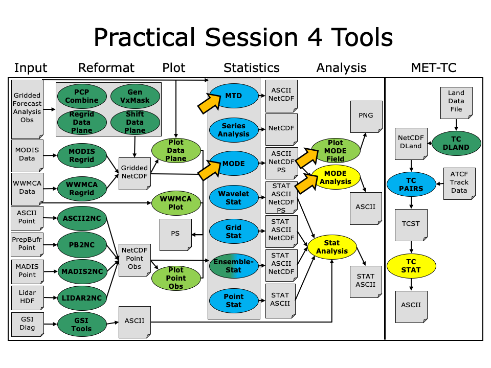
You may navigate through this tutorial by following the links at the bottom of each page or by using the menu navigation.
Since you already set up your runtime enviroment in Session 1, you should be ready to go! To be sure, run through the following instructions to check that your environment is set correctly.
Prerequisites: Verify Environment is Set Correctly
Before running these instructions, you will need to ensure that you have a few environment variables set up correctly. If they are not set correctly, these instructions will not work properly.
- Check that you have METPLUS_TUTORIAL_DIR set correctly:
If you don't see a path in your user directory output to the screen, set this environment variable in your user profile before continuing.
- Check that you have METPLUS_BUILD_BASE, MET_BUILD_BASE, and METPLUS_DATA set correctly:
echo ${MET_BUILD_BASE}
echo ${METPLUS_DATA}
If any of these variables are not set, please set them. They will be referenced throughout the tutorial.
MET_BUILD_BASE is the full path to the MET installation (/path/to/met-X.Y)
METPLUS_DATA is the location of the sample test data directory
- Check that you have loaded the MET module correctly:
You should see the usage statement for Point-Stat. The version number listed should correspond to the version listed in MET_BUILD_BASE. If it does not, you will need to either reload the met module, or add ${MET_BUILD_BASE}/bin to your PATH.
- Check that METPLUS_PARM_BASE was set correctly.
If you don't see the full path to your METplus/parm directory under the tutorial directory, please set it. See the instructions in Session 1 for more information.
- Check that the correct version of master_metplus.py is in your PATH:
If you don't see the full path to script from the shared installation, please set it. It should look the same as the output from this command:
See the instructions in Session 1 for more information.
You are now ready to move on to the next section.
MET Tool: MODE
MET Tool: MODE cindyhg Tue, 06/25/2019 - 07:58MODE Tool: General
MODE Functionality
MODE, the Method for Object-Based Diagnostic Evaluation, provides an object-based verification for comparing gridded forecasts to gridded observations. MODE may be used in a generalized way to compare any two fields containing data from which objects may be well defined. It has most commonly been applied to precipitation fields and radar reflectivity. The steps performed in MODE consist of:
- Define objects in the forecast and observation fields based on user-defined parameters.
- Compute attributes for each of those objects: such as area, centroid, axis angle, and intensity.
- For each forecast/observation object pair, compute differences between their attributes: such as area ratio, centroid distance, angle difference, and intensity ratio.
- Use fuzzy logic to compute a total interest value for each forecast/observation object pair based on user-defined weights.
- Based on the computed interest values, match objects across fields and merge objects within the same field.
- Write output statistics summarizing the characteristics of the single objects, the pairs of objects, and the matched/merged objects.
MODE may be configured to use a few different sets of logic with which to perform matching and merging. In this tutorial, we'll use the most simple approach, but users are encouraged to read Chapter 14 of the MET User's Guide for a more thorough description of MODE's capabilities.
MODE Usage
View the usage statement for MODE by simply typing the following:
| Usage: mode | ||
| fcst_file | Input gridded forecast file containing the field to be verified | |
| obs_file | Input gridded observation file containing the verifying field | |
| config_file | MODEConfig file containing the desired configuration settings | |
| [-config_merge merge_config_file] | Overrides the default fuzzy engine settings for merging within the fcst/obs fields (optional). | |
| [-outdir path] | Overrides the default output directory (optional). | |
| [-log file] | Outputs log messages to the specified file | |
| [-v level] | Level of logging | |
| [-compress level] | NetCDF compression level |
The forecast and observation fields must be on the same grid. You can use copygb to regrid GRIB1 files, wgrib2 to regrid GRIB2 files, or use the automated regridding functionality within the MET config files.
At a minimum, the input gridded fcst_file, the input gridded obs_file, and the configuration config_file must be passed in on the command line.
MODE Tool: Configure
MODE Tool: Configure cindyhg Tue, 06/25/2019 - 08:01MODE Tool: Configure
Start by making an output directory for MODE and changing directories:
cd ${METPLUS_TUTORIAL_DIR}/output/met_output/mode
The behavior of MODE is controlled by the contents of the configuration file passed to it on the command line. The default MODE configuration file may be found in the data/config/MODEConfig_default file. Prior to modifying the configuration file, users are advised to make copies of existing configuration files:
cp ${METPLUS_DATA}/met_test/scripts/config/MODEConfig_APCP_24 MODEConfig_APCP_24
cp ${METPLUS_DATA}/met_test/scripts/config/MODEConfig_RH MODEConfig_RH
We'll be using these three configuration files during this session. Open up the MODEConfig_APCP_12 file to view it.
The configuration items for MODE are used to specify how the object-based verification approach is to be performed. In MODE, as in the other MET statistics tools, you can compare any two fields. When necessary, the items in the configuration file are specified separately for the forecast and observation fields. In most cases though, users will be comparing the same forecast and observation fields. The configurable items include parameters for the following:
- The forecast and observation fields and vertical levels or accumulation intervals to be compared
- Options to mask out a portion of or threshold the raw fields
- The forecast and observation object definition parameters
- Options to filter out objects that don't meet a size or intensity criteria
- Flags to control the logic for matching/merging
- Weights to be applied for the fuzzy engine matching/merging algorithm
- Interest functions to be used for the fuzzy engine matching/merging algorithm
- Total interest threshold for matching/merging
- Various plotting options
While the MODE configuration file contains many options, beginning users will typically only need to modify a few of them. You may find a complete description of the configurable items in section 14.3.2 of the MET User's Guide. Please take some time to review them.
We'll start here using by running the configuration files we copied over, as-is.
MODE Tool: Run
MODE Tool: Run cindyhg Tue, 06/25/2019 - 08:02MODE Tool: Run
Next, run MODE three times on the command line using those three configuration files with the following commands:
${METPLUS_DATA}/met_test/out/pcp_combine/sample_fcst_12L_2005080712V_12A.nc \
${METPLUS_DATA}/met_test/out/pcp_combine/sample_obs_2005080712V_12A.nc \
MODEConfig_APCP_12 \
-outdir . \
-v 2
${METPLUS_DATA}/met_test/data/sample_fcst/2005080700/wrfprs_ruc13_24.tm00_G212 \
${METPLUS_DATA}/met_test/out/pcp_combine/sample_obs_2005080800V_24A.nc \
MODEConfig_APCP_24 \
-outdir . \
-v 2
${METPLUS_DATA}/met_test/data/sample_fcst/2005080700/wrfprs_ruc13_12.tm00_G212 \
${METPLUS_DATA}/met_test/data/sample_fcst/2005080712/wrfprs_ruc13_00.tm00_G212 \
MODEConfig_RH \
-outdir . \
-v 2
These commands make use of sample data that's distributed with the MET tarball. They run MODE on 12-hour accumulated precipitation, 24-hour accumulated precipitation, and on a field of relative humidity.
MODE Tool: Output
MODE Tool: Output cindyhg Tue, 06/25/2019 - 08:04MODE Tool: Output
The output of MODE typically consists of 4 files: 2 ASCII statistics files, 1 NetCDF object file, and 1 PostScript summary plot. The output of any of these files may be disabled using the appropriate MODE command line argument. In this example, the output is written to the current mode directory, as we requested on the command line.
The MODE output file naming convention is similar to that of the other MET tools. It contains timing information about the forecast being evaluated (forecast valid, lead, and accumulation times). If you rerun MODE on the same fields but with a slightly different configuration, the new output will override the old output, unless you redirect it to a different directory using the -outdir command line argument. You can also edit the output_prefix in the MODE configuration file to customize the output file names. The 4 MODE output files are described briefly below:
- The PostScript file ends in .ps and was described on the previous page.
- The NetCDF object file ends in _obj.nc and contains the object indices.
- The ASCII contingency table statistics file and ends in _cts.txt.
- The ASCII object statistics file ends in _obj.txt and contains all of the object and object comparison data.
You can use ghostview (gv) to look at the postscript file output from each of these three forecasts.
There are multiple pages of output. Take a moment to look them over:
-
Page 1 summarizes the entire MODE run. Thumbnail images show the input data, resolved objects, and numbers identifying each object for both the forecast and observation fields. The color indicates object matching between the forecast and observation fields. Royal blue indicates an unmatched object. The object definition information is listed at the bottom of the page, and a sorted list of total object interest is listed on the right side.
- Page 2 is an expanded view of the forecast thumbnail images.
- Page 3 is an expanded view of the observation thumbnail images.
- Page 3 is an expanded view of the observation thumbnail images.
- Page 4 has images showing the forecast objects with observation object outlines overlaid, and vice-versa.
- Page 5 shows images and statistics for matching object clusters (i.e. one or more forecast objects matching one or more observation objects). These statistics also appear in the ASCII output from MODE.
- When double-thresholding or fuzzy engine merging is enabled, additional PostScript pages are added to illustrate those methods.
You may view the output NetCDF file using ncview. Execute the following command to view the NetCDF object output of MODE:
Click through the 2D variable names in the ncview window to see plots of the four object fields in the file (NOTE: if a window pops up informing you "the min and max are both...", just Click "OK" and then the field will render). The fcst_obj_id and obs_obj_id contain the indices for the forecast and observation objects defined by MODE. The fcst_clus_id and obs_clus_idcontain indices for the matched cluster objects.
What are the benefits of spatial methods over traditional statistics? The weaknesses? What are some examples where an object-based verification would be inappropriate?
To accumulate the output of the object based verification, you use the MODE-Analysis Tool. We will use this next.
Use Case: MODE
Use Case: MODE cindyhg Tue, 06/25/2019 - 08:07METplus Use Case: MODE
The MODE use case utilizes the MET Pcp-Combine and Mode tools.
Optional: Refer to the MET Users Guide for a description of the MET tools used in this use case.
Optional: Refer to A-Z Config Glossary section of the METplus Users Guide for a reference to METplus variables used in this use case.
Setup
Create Custom Configuration File
Define a unique directory under output that you will use for this use case. Create a configuration file to override OUTPUT_BASE to that directory.
Set OUTPUT_BASE to contain a subdirectory specific to the Mode use case. Make sure to put it under the [dir] section.
OUTPUT_BASE = {ENV[METPLUS_TUTORIAL_DIR]}/output/mode
Using this custom configuration file and the Mode use case configuration files that are distributed with METplus, you should be able to run the use case using the sample input data set without any other changes.
Review Use Case Configuration File: hrefmean-vs-mrms-qpe.conf
Open the file and look at all of the configuration variables that are defined.
Note that variables in hrefmean-vs-mrms-qpe.conf reference other config variables that have been defined in other configuration files. For example:
This references INPUT_BASE which is the METplus data configuration file (metplus_config/metplus_data.conf). METplus config variables can reference other config variables even if they are defined in a config file that is read afterwards.
Run METplus
Run the following command:
METplus is finished running when control returns to your terminal console and you see the following text:
Review the Output Files
You should have output files in the following directories:
- mode_HREF_MEAN_APCP_vs_MRMS_QPE_P06M_NONE_A06_000000L_20170622_000000V_NAA_R1_T1_cts.txt
- mode_HREF_MEAN_APCP_vs_MRMS_QPE_P06M_NONE_A06_000000L_20170622_000000V_NAA_R1_T1_obj.nc
- mode_HREF_MEAN_APCP_vs_MRMS_QPE_P06M_NONE_A06_000000L_20170622_000000V_NAA_R1_T1_obj.txt
- mode_HREF_MEAN_APCP_vs_MRMS_QPE_P06M_NONE_A06_000000L_20170622_000000V_NAA_R1_T1.ps
Take a look at some of the files to see what was generated.
Review the Log Files
Log files for this run are found in ${METPLUS_TUTORIAL_DIR}/output/mode/logs. The filename contains a timestamp of the current day.
NOTE: If you ran METplus on a different day than today, the log file will correspond to the day you ran. Remove the date command and replace it with the date you ran if that is the case.
Review the Final Configuration File
The final configuration file is metplus_final.conf. This contains all of the configuration variables used in the run.
MET Tool: MTD
MET Tool: MTD cindyhg Tue, 06/25/2019 - 08:13MODE-Time-Domain: General
MODE-Time-Domain Functionality
The MODE-Time-Domain (MTD) tool was added in MET version 6.0. It applies an object-based verification technique in comparing a gridded forecast to a gridded analysis. It defines 3-dimensional space/time objects, tracking 2-dimensional objects through time. It writes summary object information to ASCII statistics files and writes object fields to NetCDF format. The MTD tool can be used to quantify the duration of events and timinig errors.
MODE-Time-Domain Usage
View the usage statement for MODE-Time-Domain by simply typing the following:
The forecast and observation fields must be on the same grid. You can use copygb to regrid GRIB1 files, wgrib2 to regrid GRIB2 files, or use the automated regridding functionality within the MET config files.
At a minimum, the -fcst and -obs options must be used to specify the data to be processed. Alternatively, the -single option specifies that MTD should be run on a single dataset. The -config option specifies the name of the configuration file.
MTD: Configure
MTD: Configure cindyhg Tue, 06/25/2019 - 08:15MTD: Configure
Start by making an output directory for MTD and changing directories:
cd ${METPLUS_TUTORIAL_DIR}/output/met_output/mtd
The behavior of MTD is controlled by the contents of the configuration file passed to it on the command line. The default MTD configuration file may be found in the data/config/MTDConfig_default file. Prior to modifying the configuration file, users are advised to make a copy of the default:
The configuration items for MTD are used to specify how the space-time-object-based verification approach is to be performed. Just as MODE may be used to compare any two fields, the same is true of MTD. When necessary, the items in the configuration file are specified separately for the forecast and observation fields. In most cases though, users will be comparing the same forecast and observation fields. The configurable items include specifications for the following:
- The verification domain.
- The forecast and observation fields and vertical levels or accumulation intervals to be compared.
- The forecast and observation object definition parameters.
- Options to filter out objects that don't meet a minimum volume.
- Matching/merging weights and interest functions.
- Total interest threshold for matching/merging.
- Flags to control output files.
For this tutorial, we'll configure MTD to process the same series of data we ran through the Series-Analysis tool. Just like MODE, MTD compares a single forecast field to a single observation field in each run.
Open up the MTDConfig_tutorial file for editing with the text editor of your choice and edit it as follows:
Set the fcst dictionary as follows:
field = {
name = "APCP";
level = "A03";
}
conv_radius = 2;
conv_thresh = >=2.54;
}
Set the obs dictionary as follows:
field = {
name = "APCP_03";
level = "(*,*)";
}
conv_radius = 2;
conv_thresh = >=2.54;
}
Set:
To retain all objects regardless of their volume.
Save and close this file.
MTD: Run
MTD: Run cindyhg Tue, 06/25/2019 - 08:16MTD: Run
First, we need to prepare our observations by putting 1-hourly StageII precipitation forecasts into 3-hourly buckets. Create an output directory:
Run the following PCP-Combine commands to prepare the observations:
sample_obs/ST2ml_3h/sample_obs_2005080703V_03A.nc \
-pcpdir ${METPLUS_DATA}/met_test/data/sample_obs/ST2ml
sample_obs/ST2ml_3h/sample_obs_2005080706V_03A.nc \
-pcpdir ${METPLUS_DATA}/met_test/data/sample_obs/ST2ml
sample_obs/ST2ml_3h/sample_obs_2005080709V_03A.nc \
-pcpdir ${METPLUS_DATA}/met_test/data/sample_obs/ST2ml
sample_obs/ST2ml_3h/sample_obs_2005080712V_03A.nc \
-pcpdir ${METPLUS_DATA}/met_test/data/sample_obs/ST2ml
sample_obs/ST2ml_3h/sample_obs_2005080715V_03A.nc \
-pcpdir ${METPLUS_DATA}/met_test/data/sample_obs/ST2ml
sample_obs/ST2ml_3h/sample_obs_2005080718V_03A.nc \
-pcpdir ${METPLUS_DATA}/met_test/data/sample_obs/ST2ml
sample_obs/ST2ml_3h/sample_obs_2005080721V_03A.nc \
-pcpdir ${METPLUS_DATA}/met_test/data/sample_obs/ST2ml
sample_obs/ST2ml_3h/sample_obs_2005080800V_03A.nc \
-pcpdir ${METPLUS_DATA}/met_test/data/sample_obs/ST2ml
Rather than listing 8 input forecast and observation files on the command line, we will write them to a file list first. Since the 0-hour forecast does not contain 3-hourly accumulated precip, we will exclude that from the list. We will use the 3-hourly APCP output from PCP-Combine that we prepared above:
ls -1 sample_obs/ST2ml_3h/sample_obs* > obs_file_list
Next, run the following MTD command:
-fcst fcst_file_list \
-obs obs_file_list \
-config MTDConfig_tutorial \
-outdir . \
-v 2
Just as with MODE, MTD applies a convolution operation to smooth the data. However, there are two important differences. In MODE, the convolution shape is a circle (radius = conv_radius). In MTD, the convolution shape is a square (width = 2*conv_radius+1) and for time t, the values in that square are averaged for times t-1, t, and t+1. Convolving in space plus time enables MTD to identify more continuous space-time objects.
If your data has high enough time frequency that the features at one timestep overlap those at the next timestep, it may be well-suited for MTD.
MTD: Output
MTD: Output cindyhg Tue, 06/25/2019 - 08:17MTD: Output
The MTD output typically consists of 6 files: 5 ASCII statistics files and 1 NetCDF object file. MTD does not create any graphical output. In this example, the output is written to the current mtd directory as we requested on the command line.
The MTD output file naming convention begins with mtd_ followed by the last valid time it encountered. The output file names may be modified using the output_prefix option in the configuration file which should be used to prevent the output of one run from over-writing the output of a previous run. The 6 MTD output files are described briefly below:
- The NetCDF object file ends in .nc and contains gridded fields of the raw data, simple object indices, and cluster object indices for each forecast and observed timestep.
- The ASCII file ending with _2D.txt contains many columns similar to the output of MODE. This data summarizes the 2-dimensional object attributes for each individual time slice of the 3D forecast and observation objects.
- The ASCII files ending with _single_simple.txt and _single_cluster.txt contain 3D space-time attributes for simple and cluster objects, respectively.
- The ASCII files ending with _pair_simple.txt and _pair_cluster.txt contain 3D space-time attributes for pairs of simple and cluster objects, respectively.
Use the ncview utility to view the NetCDF object output of MTD:
Select the variable named fcst_raw and click the time index to advance through the timesteps. Now, do the same for the fcst_object_id variable. Notice that the objects are defined in the active areas in the raw fields. Also notice some features merging (i.e. combining) as time passes while other features split (i.e. break apart). While they may be disconnected at a particular timestep, they remain part of the same space-time object.
Next, explore the ASCII output files and pay close attention to the header columns. Notice the generalization of the 2D MODE object attributes to 3 dimensions. Area meausure become volume. MTD measure the object speed. Each object has a begining and ending time.
Use Case: MTD
Use Case: MTD cindyhg Tue, 06/25/2019 - 08:20METplus Use Case: MTD
Reference Material
The MTD (Mode Time Domain) use case utilizes the MET MTD tools.
Optional: Refer to the MET Users Guide for a description of the MET tools used in this use case.
Optional: Refer to the A-Z Config Glossary section of the METplus Users Guide for a reference to METplus variables used in this use case.
Setup
Create Custom Configuration File
Define a unique directory under output that you will use for this use case. Create a configuration file to override OUTPUT_BASE to that directory.
Set OUTPUT_BASE to contain a subdirectory specific to the MTD use case. Make sure to put it under the [dir] section.
OUTPUT_BASE = {ENV[METPLUS_TUTORIAL_DIR]}/output/mtd
Using this custom configuration file and the MTD use case configuration files that are distributed with METplus, you should be able to run the use case using the sample input data set without any other changes.
Review Use Case Configuration File: phpt-vs-qpe.conf
Open the file and look at all of the configuration variables that are defined.
Note that variables in phpt-vs-qpe.conf reference other config variables that have been defined in other configuration files. For example:
This references INPUT_BASE which is set in the METplus data configuration file (metplus_config/metplus_data.conf). METplus config variables can reference other config variables even if they are defined in a config file that is read afterwards.
Run METplus
Run the following command:
METplus is finished running when control returns to your terminal console and you see the following text:
Review the Output Files
You should have output files in the following directories:
- mtd_PROB_PHPT_APCP_vs_QPE_P01M_NONE_A01_20170510_040000V_2d.txt
- mtd_PROB_PHPT_APCP_vs_QPE_P01M_NONE_A01_20170510_040000V_3d_pair_cluster.txt
- mtd_PROB_PHPT_APCP_vs_QPE_P01M_NONE_A01_20170510_040000V_3d_pair_simple.txt
- mtd_PROB_PHPT_APCP_vs_QPE_P01M_NONE_A01_20170510_040000V_3d_single_cluster.txt
- mtd_PROB_PHPT_APCP_vs_QPE_P01M_NONE_A01_20170510_040000V_3d_single_simple.txt
- mtd_PROB_PHPT_APCP_vs_QPE_P01M_NONE_A01_20170510_040000V_obj.nc
Take a look at some of the files to see what was generated.
Open the output NetCDF file with ncview to look at the data:
Click on the buttons in the Var: section (i.e. fcst_raw) to view the fields.
Open an output text file to view the contents:
Review the Log Files
Log files for this run are found in ${METPLUS_TUTORIAL_DIR}/output/mtd/logs. The filename contains a timestamp of the current day.
NOTE: If you ran METplus on a different day than today, the log file will correspond to the day you ran. Remove the date command and replace it with the date you ran if that is the case.
Review the Final Configuration File
The final configuration file is metplus_final.conf. This contains all of the configuration variables used in the run.
Additional Exercises
Additional Exercises cindyhg Tue, 06/25/2019 - 08:25End of Practical Session 4
Congratulations! You have completed Session 4!
If you have extra time, you may want to try these additional METplus exercises.
EXERCISE 4.1: mtd_skip - Change Forecast Lead List to See METplus Skip Files
Instructions: Modify the METplus configuration files to change the forecast leads that are processed by MTD. Following these instructions will give you more insight on how METplus configures MTD.
Change LEAD_SEQ to process forecast leads 1-4
less ${METPLUS_TUTORIAL_DIR}/output/exercises/mtd_skip/stage/file_lists/201705100300_mtd_obs_P01M_NONE.txt
ls ${METPLUS_DATA}/mode/QPE_Data/20170510
EXERCISE 4.2: unzip - Change Forecast Lead List to See METplus Unzip
Instructions: Modify the METplus configuration files to change the forecast leads that are processed by MTD. Following these instructions will give you more insight on how METplus configures MTD.
Open mtd.unzip.conf with an editor and changes values.
Now look at the file list that were generated by METplus for MTD forecast files
If you look in the data directories for this run, you will see that the 6 hour forecast file is gzipped.
Session 5: Trk&Int/Feature Relative
Session 5: Trk&Int/Feature Relative admin Wed, 06/12/2019 - 16:59During this practical session, you will run the tools indicated below:

You may navigate through this tutorial by following the links at the bottom of each page or by using the menu navigation.
Since you already set up your runtime enviroment in Session 1, you should be ready to go! To be sure, run through the following instructions to check that your environment is set correctly.
Prerequisites: Verify Environment is Set Correctly
Before running these instructions, you will need to ensure that you have a few environment variables set up correctly. If they are not set correctly, these instructions will not work properly.
- Check that you have METPLUS_TUTORIAL_DIR set correctly:
If you don't see a path in your user directory output to the screen, set this environment variable in your user profile before continuing.
- Check that you have METPLUS_BUILD_BASE, MET_BUILD_BASE, and METPLUS_DATA set correctly:
echo ${MET_BUILD_BASE}
echo ${METPLUS_DATA}
If any of these variables are not set, please set them. They will be referenced throughout the tutorial.
MET_BUILD_BASE is the full path to the MET installation (/path/to/met-X.Y)
METPLUS_DATA is the location of the sample test data directory
- Check that you have loaded the MET module correctly:
You should see the usage statement for Point-Stat. The version number listed should correspond to the version listed in MET_BUILD_BASE. If it does not, you will need to either reload the met module, or add ${MET_BUILD_BASE}/bin to your PATH.
- Check that METPLUS_PARM_BASE was set correctly.
If you don't see the full path to your METplus/parm directory under the tutorial directory, please set it. See the instructions in Session 1 for more information.
- Check that the correct version of master_metplus.py is in your PATH:
If you don't see the full path to script from the shared installation, please set it. It should look the same as the output from this command:
See the instructions in Session 1 for more information.
You are now ready to move on to the next section.
MET Tool: TC-Pairs
MET Tool: TC-Pairs cindyhg Mon, 06/24/2019 - 11:18TC-Pairs Tool: General
TC-Pairs Functionality
The TC-Pairs tool provides position and intensity information for tropical cyclone forecasts in Automated Tropical Cyclone Forecast System (ATCF) format. Much like the Point-Stat tool, TC-Pairs produces matched pairs of forecast model output and an observation dataset. In the case of TC-Pairs, both the model output and observational dataset (or reference forecast) must be in ATCF format. TC-Pairs produces matched pairs for position errors, as well as wind, sea level pressure, and distance to land values for each input dataset.
TC-Pairs input data format
As mentioned above, the input to TC-Pairs is two ATCF format files, in addition to the distance_to_land.nc file generated with the TC-Dland tool. The ATCF file format is a comma-separated ASCII file containing the following fields:
| Basin | basin | |
| CY | annual cyclone number (1-99) | |
| YYYYMMDDHH | Date - Time - Group | |
| TECHNUM/MIN | Objective sorting technique number, minutes in Best Track | |
| TECH | acronym for each objective technique | |
| TAU | forecast period | |
| LatN/S | Latitude for the date time group | |
| LonE/W | Longitude for date time group | |
| VMAX | Maximum sustained wind speed | |
| MSLP | Minimum sea level pressure | |
| TY | Highest level of tropical cyclone development | |
| RAD | wind intensity for the radii at 34, 50, 64 kts | |
| WINDCODE | radius code | |
| RAD1 | full circle radius of wind intensity, 1st quadrant wind intensity | |
| RAD2 | radius of 2nd quadrant wind intensity | |
| RAD3 | radius of 3rd quadrant wind intensity | |
| RAD4 | radius of 4th quadrant wind intensity | |
| ... |
These are the first 17 columns in the ATCF file format. MET-TC requires the input file has all 17 comma-separated columns present (although valid data is not required). For a full list of the columns as well as greater detail on the file format, see: http://www.nrlmry.navy.mil/atcf_web/docs/database/new/abdeck.txt
Model data must be run through a vortex tracking algorithm prior to becoming input for MET-TC. Running a vortex tracker is outside to scope of this tutorial, however a freely available and supported vortex tracking software is available at: http://www.dtcenter.org/HurrWRF/users/downloads/index.php
If users choose to use operational model data for input to MET-TC, all U.S. operational model output in ATCF format can be found at: ftp://ftp.nhc.noaa.gov/atcf/archive. Finally, the most common use of MET-TC is to use the best track analysis (used as observations) to generate pairs between the model forecast and the observations. Best track analyses can be found at the same link as the operational model output.
Open files aal112017.dat (model data) and bal112017.dat (BEST track). Take a look at the columns and gain familiarity with ATCF format. These files are input ATCF files for TC-Pairs.
In addition to the files above, data from five total storms over hurricane seasons 2011-2012 in the AL basin will be used to run TC-Pairs. Rather than running a single storm, these storms were chosen to provide a larger sample size to provide more robust statistics.
- aal092011: Irene
- aal182011: Rina
- aal052012: Ernesto
- aal092012: Isaac
- aal182012: Sandy
TC-Pairs Tool: General
TC-Pairs Tool: General cindyhg Mon, 06/24/2019 - 11:56TC-Pairs Tool: General
TC-Pairs Usage
View the usage statement for TC-Pairs by simply typing the following:
| Usage: tc_pairs | ||
| -adeck source | Input ATCF format track files | |
| -edeck source | Input ATCF format ensemble probability files | |
| -bdeck source | Input ATCF format observation (or reference forecast) file path/name | |
| -config file | Configuration file | |
| [-out_base] | path of output file base | |
| [-log_file] | name of log associated with tc_pairs output | |
| [-v level] | Level of logging (optional) |
At a minimum, the input ATCF format -adeck (or -edeck) source, the input ATCF format -bdeck source, and the configuration -config file must be passed in on the command line.
The -adeck, -edeck, and -edeck options can be set to either a specific file name or a top-level directory which will be searched for files ending in ".dat".
TC-Pairs Tool: Configure
TC-Pairs Tool: Configure cindyhg Mon, 06/24/2019 - 11:57TC-Pairs Tool: Configure
Start by making an output directory for TC-Pairs and changing directories:
cd ${METPLUS_TUTORIAL_DIR}/output/met_output/tc_pairs
Like the Point-Stat tool, the TC-Pairs tool is controlled by the contents of the configuration file passed to it on the command line. The default TC-Pairs configuration file may be found in the data/config/TCPairsConfig_default file.
The configurable items for TC-Pairs are used to specify which data are ingested and how the input data are filtered. The configurable items include specifications for the following:
- All model names to include in matched pairs
- Storms to include in verification: parsed by storm_id, basin, storm_name, cyclone
- Date/Time/Space restrictions: initialization time, valid time, lead time, masking
- User defined consensus forecasts
- Thresholds over watch/warning status of storm
The first step is to set-up the configuration file. Keep in mind, TC-Pairs should be run with the largest desired sample in mind to minimize re-running this tool! First, make a copy of the default:
Next, open up the TCPairsConfig_tutorial_run file for editing and modify it as follows:
Set:
basin = [ "AL" ];
To identify the models to we want to verify, as well as the basin. The three models identified are all U.S. operational models: HWRF, GFS (AVNO), and GFDL. Any field left blank will assume no restictions.
Set:
{
name = "CONS";
members = [ "HWRF", "AVNO", "GFDL" ];
required = [ false, false, false ];
min_req = 2;
}
];
To compute a user defined consensus named "CONS". The membership of the consensus are the three listed models, none are required, but 2 must be present to calculate the consensus.
Set:
To only keep pairs that are the intersection of the model forecast and observation.
Next, save the TCPairsConfig_tutorial_run file and exit the text editor.
This run uses the default distance to land output file. Run ncview to see it:
Water points have distance to land values greater than 0 while land points have distances <= 0.
TC-Pairs Tool: Run
TC-Pairs Tool: Run cindyhg Mon, 06/24/2019 - 11:58TC-Pairs Tool: Run
Next, run TC-Pairs to compare all three ATCF forecast models specified in configuration file to the ATCF format best track analysis. Run the following command line:
-adeck ${METPLUS_DATA}/met_test/atcf_data/aal*dat \
-bdeck ${METPLUS_DATA}/met_test/atcf_data/bal*dat \
-config TCPairsConfig_tutorial_run \
-out tc_pairs \
-v 2
TC-Pairs is now grabbing the model data we requested in the configuration file, generating the consensus, and performing the additional filtering criteria. It should take only a few minutes to run. You should see several status messages printed to the screen to indicate progress.
If you are running many models over many storms/seasons, it is best to run TC-Pairs using a script to call TC-Pairs for each storm. This avoids potential memory issues when parsing very large datasets.
TC-Pairs Tool: Output
TC-Pairs Tool: Output cindyhg Mon, 06/24/2019 - 11:59TC-Pairs Tool: Output
The output of TC-Pairs is an ASCII file containing matched pairs for each of the models requested. In this example, the output is written to the tc_pairs.tcst file as we requested on the command line. This output file is in TCST format, which is similar to the STAT output from the Point-Stat and Grid-Stat tools. For more header information on the TCST format, see section 19.2.3 of the MET User's Guide.
Remember to configure your text editor to NOT use dynamic word wrapping. The files will be much easier to read that way:
- In the kwrite editor, select Settings->Configure Editor, de-select Dynamic Word Wrap and click OK.
- In the vi editor, type the command :set nowrap. To set this as the default behavior, run the following command:
echo "set nowrap" >> ~/.exrc
Open tc_pairs.tcst
- Notice this is a simple ASCII file with rows for each matched pair for a single valid time..
- Any field that has A in the column name (such as AMAX_WIND, ALAT) indicate the model forecast.
- Any field that has B in the column name (such as BMAX_WIND, BLAT) indicate the observation field (Best Track).
- The TK_ERR, X_ERR, Y_ERR, ALTK_ERR, CRTK_ERR columns are calculated track error, X component position error, Y component postion error, along track error, and cross track error, respectively.
- Columns 34-63 are the 34-, 50-, and 64-kt wind radii for each quadrant.
MET Tool: TC-Stat
MET Tool: TC-Stat cindyhg Mon, 06/24/2019 - 12:01TC-Stat Tool: General
TC-Stat Functionality
The TC-Stat tool reads the .tcst output file(s) of the TC-Pairs tool. This tools provides the ability to further filter the TCST output files as well as summarize the statistical information. The TC-Stat tool reads .tcst files and runs one or more analysis jobs on the data. TC-Stat can be run by specifying a single job on the command line or multiple jobs using a configuration file. The TC-Stat tool is very similar to the Stat-Analysis tool. The two analysis job types are summarized below:
- The filter job simply filters out lines from one or more TCST files that meet the filtering options specified.
- The summary job operates on one column of data from TCST file. It produces summary information for that column of data: mean, standard deviation, min, max, and the 10th, 25th, 50th, 75th, and 90th percentiles, independence time, and frequency of superior performance.
- The rirw job identifies rapid intensification or weakening events in the forecast and analysis tracks and applies categorical verification methods.
- The probrirw job applies probabilistic verification methods to evaluate probability of rapid inensification forecasts found in edeck's.
TC-Stat Usage
View the usage statement for TC-Stat by simply typing the following:
| Usage: tc_stat | ||
| -lookin path | TCST file or top-level directory containing TCST files (where TC-Pairs output resides). It allows the use of wildcards (at least one tcst file is required). | |
| [-out file] | Output path or specific filename to which output should be written rather than the screen (optional). | |
| [-log file] | Outputs log messages to the specified file | |
| [-v level] | Level of logging | |
| [-config config_file] | [JOB COMMAND LINE] (Note: "|" means "or") | ||
| [-config config_file] | TCStat config file containing TC-Stat jobs to be run. | |
| [JOB COMMAND LINE] | Arguments necessary to perform a TC-Stat job. |
At a minimum, you must specify at least one directory or file in which to find TCST data (using the -lookin path command line option) and either a configuration file (using the -config config_file command line option) or a job command on the command line.
TC-Stat Tool: Configure
TC-Stat Tool: Configure cindyhg Mon, 06/24/2019 - 12:02TC-Stat Tool: Configure
Start by making an output directory for TC-Stat and changing directories:
cd ${METPLUS_TUTORIAL_DIR}/output/met_output/tc_stat
The behavior of TC-Stat is controlled by the contents of the configuration file or the job command passed to it on the command line. The default TC-Stat configuration may be found in the data/config/TCStatConfig_default file. Make a copy of the default configuration file and make following modifications:
Open up the TCStatConfig_tutorial file for editing with your preferred text editor.
Set:
bmodel = [ "BEST" ];
event_equal = TRUE;
To only parse over two of the three model names in the tc_pairs.tcst file. The event_equal=TRUE flag will keep pairs that are in both HWRF and GFDL pairs.
Many of the filter options are left blank, indicating TC-Stat should parse over all available fields. You will notice many more available filter options beyond what was available with the TCPairsConfig.
Now, scroll all the way to the bottom of the TCStatConfig, and you will find the jobs[] section. Edit this section as follows:
TC-Stat: Run on TC-Pairs output
TC-Stat: Run on TC-Pairs output cindyhg Mon, 06/24/2019 - 12:03TC-Stat: Run on TC-Pairs output
Run the TC-Stat using the following command:
-lookin ../tc_pairs/tc_pairs.tcst \
-config TCStatConfig_tutorial -v 3
Open the output file tc_stat.tcst. We can see that this filter job simply event equalized the two models specified in amodel.
Let's try to filter further, this time using the command line rather than the configuration file:
-job filter -lookin ../tc_pairs/tc_pairs.tcst \
-dump_row tc_stat2.tcst \
-water_only TRUE \
-column_str LEVEL HU,TS,TD,SS,SD \
-event_equal TRUE \
-match_points TRUE -v 3
Here, we ran a filter job at the command line: only keeping tracks over water (not encountering land) and with categories Hurricane (HU), Tropical Storm (TS), Tropical Depression (TD), Subtropical Storm (SS), and Subtropical Depression (SD).
Open the output file tc_stat2.tcst: notice fewer lines have been kept. Look at the "LEVEL" column ... note all the non-tropical and subtropical level classifications have been filtered out of the sample.
Also, find the columns ADLAND and BDLAND. All these values are now positive, meaning the tracks over land (negative values) have been filtered.
With the filtering jobs mastered, lets give the second type of job - summary jobs - a try!
TC-Stat: Run on TC-Pairs output
TC-Stat: Run on TC-Pairs output cindyhg Mon, 06/24/2019 - 12:03TC-Stat: Run on TC-Pairs output
Now, we will run a summary job using TC-Stat on the command line using the following command:
-job summary -lookin ../tc_pairs/tc_pairs.tcst \
-amodel HWRF,GFDL \
-by LEAD,AMODEL \
-column TK_ERR \
-event_equal TRUE \
-out tc_stat_summary.tcst
Open up the file tc_stat_summary.tcst. Notice this output is much different from the filter jobs.
The track data is event equalized for the HWRF and GFDL models, and summary statistics are produced for the TK_ERR column for each model by lead time.
TC-Stat: Plotting with R
TC-Stat: Plotting with R cindyhg Mon, 06/24/2019 - 12:03TC-Stat: Plotting with R
In this section, you will use the R statistics software package to produce a plot of a few results. R was introduced in practical session 1.
export MET_BASE=${MET_INSTALL_DIR}/share/met
Rscript ${MET_BASE}/Rscripts/plot_tcmpr.R
The TC-Stat tool can be called from the Rscript to do additional filter jobs on the TCST output from TC-Pairs. This can be done on the command line by calling a filter job (following tc-stat), or a configuraton file can be used to select filtering criteria. A default configuration file can be found in Rscripts/include/plot_tcmpr_config_default.R.
The configuration file also includes various plot types to generate: MEAN, MEDIAN, SCATTER, REFPERF, BOXPLOT, and RANK. All of the plot commands can be called on the command line as well as with the configuration file. Plots are configurable (title, colors, axis labels, etc) either by modifying the configuration file or setting options on the command line. To run from the command line:
-lookin ../tc_pairs/tc_pairs.tcst \
-filter "-amodel HWRF,CONS" \
-dep "TK_ERR" \
-series AMODEL HWRF,CONS \
-plot MEAN,BOXPLOT,RANK \
-outdir .
This plots the track error for two models: HWRF and CONS. CONS is the user defined consensus you generated in TC-Pairs.
Next, open up the output *png files:
display TK_ERR_mean.png &
display TK_ERR_rank.png &
The script produces the three plot types called in the configuration file:
- Boxplot showing distribution of errors for a homogeneous sample of the two models (TK_ERR_boxplot.png).
- Mean Errors with 95% CI for the same sample (TK_ERR_mean.png).
- Rank plot indicating performance of HWRF model relative to CONS (TK_ERR_rank.png).
Use Case: Track and Intensity
Use Case: Track and Intensity cindyhg Mon, 06/24/2019 - 14:24METplus Use Case: Track and Intensity TCMPR (Tropical Cyclone Matched Pair) Plotter
This is a wrapper to the MET plot_tcmpr.R Rscript.
Setup
Create Custom Configuration File
Define a unique directory under output that you will use for this use case. Create a configuration file to override OUTPUT_BASE to that directory.
Set OUTPUT_BASE to contain a subdirectory specific to the Track and Intensity use case. Make sure to put it under the [dir] section.
OUTPUT_BASE = {ENV[METPLUS_TUTORIAL_DIR]}/output/track_and_intensity
Using this custom configuration file and the Track and Intensity use case configuration files that are distributed with METplus, you should be able to run the use case using the sample input data set without any other changes.
Review: Take a look at the following settings.
The default image resolution for the plot_tcmpr.R Rscript is set to 300, for print quality, but quite large for display purposes. The following is an R config file that is passed to the Rscript and changes the default and reduces the image size. It is a simple one line file, but go and take a look.
The plot_tcmpr.R script knows to read this tcmpr_customize.conf R config file since it is defined in the track_and_intensity.conf file.
These are some common settings for the track and intensity use case. These have already been defined in the track_and_intensity.conf file. If desired or needed, these can be overridden in this track and intensity use case conf files
TCMPR_DATA - the path to the input data, in this example, we are using the data in the TC_PAIRS_DIR directory.
MODEL_DATA_DIR - path to the METplus input data.
TRACK_DATA_DIR - path to the METplus input data.
Optional, Refer to the TC-Stat tool example section of the MET Users Guide for a description of plot_tcmpr.R
If you wish, refer to Table 19.2 Format Information for TCMPR output line type, for a tabular description of the TC-Pairs output TCST format. After running this Track and Intensity example, you can view the TC-Pairs TCST output files generate by this example under your ${METPLUS_TUTORIAL_DIR}/output/track_and_intensity/tc_pairs directory while comparing to the information in the table.
The tcmpr defaults are used for any conf settings left as, unset, For example as: XLAB =
The current settings in the conf files are ok and no changes are required. However, after running the exercise feel free to experiment with these settings.
The R script that Track and Intensity runs is located in the MET installation; share/met/Rscripts/plot_tcmpr.R. The usage statement with a short description of the options for plot_tcmpr.R can be obtained by typing: Rscript plot_tcmpr.R with no additional arguments. The usage statement can be helpful when setting some of the option in METplus, below is a description of these settings.
- CONFIG_FILE is a plotting configuration file
PREFIX is the output file name prefix.
TITLE overrides the default plot title. Bug: CAN_NOT_HAVE_SPACES
SUBTITLE overrides the default plot subtitle.
XLAB overrides the default plot x-axis label.
YLAB overrides the default plot y-axis label.
XLIM is the min,max bounds for plotting the X-axis.
YLIM is the min,max bounds for plotting the Y-axis.
FILTER is a list of filtering options for the tc_stat tool.
FILTERED_TCST_DATA_FILE is a tcst data file to be used instead of running the tc_stat tool.
DEP_VARS is a comma-separated list of dependent variable columns to plot.
SCATTER_X is a comma-separated list of x-axis variable columns to plot.
SCATTER_Y is a comma-separated list of y-axis variable columns to plot.
SKILL_REF is the identifier for the skill score reference.
LEGEND is a comma-separted list of strings to be used in the legend.
LEAD is a comma-separted list of lead times (h) to be plotted.
RP_DIFF is a comma-separated list of thresholds to specify meaningful differences for the relative performance plot.
DEMO_YR is the demo year
HFIP_BASELINE is a string indicating whether to add the HFIP baseline and which version (no, 0, 5, 10 year goal)
FOOTNOTE_FLAG to disable footnote (date).
PLOT_CONFIG_OPTS to read model-specific plotting options from a configuration file.
SAVE_DATA to save the filtered track data to a file instead of deleting it.
PLOT_TYPES- is a comma-separated list of plot types to create:
BOXPLOT, POINT, MEAN, MEDIAN, RELPERF, RANK, SKILL_MN, SKILL_MD
-for this example, set to MEAN,MEDIAN to generate MEAN and MEDIAN plots.
SERIES
- is the column whose unique values define the series on the plot,
optionally followed by a comma-separated list of values, including:
ALL, OTHER, and colon-separated groups.
SERIES_CI
- is a list of true/false for confidence intervals.
optionally followed by a comma-separated list of values, including:
ALL, OTHER, and colon-separated groups.
- is a comma-separated list of plot types to create:
Run METplus: Run Track and Intensity use case.
Examples: Run the track and intensity plotting script
Generates plots using the MET plot_tcmpr.R Rscript.
Example:
In this case we are generating the BOXPLOT, MEAN, and MEDIAN plots.
Run the following command:
The following directory lists the files generated from running these use cases:
AMAX_WIND-BMAX_WIND_median.png
AMSLP-BMSLP_mean.png
AMSLP-BMSLP_median.png
TK_ERR_boxplot.png
TK_ERR_boxplot.log
TK_ERR_mean.png
TK_ERR_median.png
To view the images generated by running these examples, use the display command.
cd to your OUTPUT_BASE/tcmpr_plots directory, depending on your setting it may be here.
display AMAX_WIND-BMAX_WIND_mean.png
MET Tool: Series-Analysis
MET Tool: Series-Analysis cindyhg Mon, 06/24/2019 - 14:28Series-Analysis Tool: General
Series-Analysis Functionality
The Series-Analysis Tool accumulates statistics separately for each horizontal grid location over a series. Usually, the series is defined as a time series, however any type of series is possible, including a series of vertical levels. This differs from the Grid-Stat tool in that Grid-Stat computes statistics aggregated over a spatial masking region at a single point in time. The Series-Analysis Tool computes statistics for each individual grid point and can be used to quantify how the model performance varies over the domain.
Series-Analysis Usage
View the usage statement for Series-Analysis by simply typing the following:
| Usage: series_analysis | ||
| -fcst file_1 ... file_n | Gridded forecast files or ASCII file containing a list of file names. | |
| -obs file_1 ... file_n | Gridded observation files or ASCII file containing a list of file names. | |
| [-both file_1 ... file_n] | Sets the -fcst and -obs options to the same list of files (e.g. the NetCDF matched pairs files from Grid-Stat). |
|
| [-paired] | Indicates that the -fcst and -obs file lists are already matched up (i.e. the n-th forecast file matches the n-th observation file). |
|
| -out file | NetCDF output file name for the computed statistics. | |
| -config file | SeriesAnalysisConfig file containing the desired configuration settings. | |
| [-log file] | Outputs log messages to the specified file | |
| [-v level] | Level of logging (optional). | |
| [-compress level] | NetCDF compression level (optional). |
At a minimum, the -fcst, -obs (or -both), -out, and -config settings must be passed in on the command line. All forecast and observation fields must be interpolated to a common grid prior to running Series-Analysis.
Series-Analysis Tool: Configure
Series-Analysis Tool: Configure johnhg Thu, 07/25/2019 - 23:03Series-Analysis Tool: Configure
Start by making an output directory for Series-Analysis and changing directories:
cd ${METPLUS_TUTORIAL_DIR}/output/met_output/series_analysis
The behavior of Series-Analysis is controlled by the contents of the configuration file passed to it on the command line. The default Series-Analysis configuration file may be found in the data/config/SeriesAnalysisConfig_default file. Prior to modifying the configuration file, users are advised to make a copy of the default:
The configurable items for Series-Analysis are used to specify how the verification is to be performed. The configurable items include specifications for the following:
- The forecast fields to be verified at the specified vertical level or accumulation interval.
- The threshold values to be applied.
- The area over which to limit the computation of statistics - as predefined grids or configurable lat/lon polylines.
- The confidence interval methods to be used.
- The smoothing methods to be applied.
- The types of statistics to be computed.
You may find a complete description of the configurable items in section 13.2.3 of the MET User's Guide. Please take some time to review them.
For this tutorial, we'll run Series-Analysis to verify a time series of 3-hour accumulated precipitation. We'll use GRIB1 for the forecast files and NetCDF for the observation files. Since the forecast and observations are different file formats, we'll specify the name and level information for them slightly differently.
Open up the SeriesAnalysisConfig_tutorial file for editing with your preferred text editor and edit it as follows:
- Set the fcst dictionary to
fcst = {
field = [
{
name = "APCP";
level = [ "A3" ];
}
];
}To request the GRIB abbreviation for precipitation (APCP) accumulated over 3 hours (A3).
- Delete obs = fcst; and insert
obs = {
field = [
{
name = "APCP_03";
level = [ "(*,*)" ];
}
];
}To request the NetCDF variable named APCP_03 where its two dimensions are the gridded dimensions (*,*).
- Set
cat_thresh = [ >0.0, >=5.0 ];To define the categorical thresholds of interest. By defining this at the top level of config file context, these thresholds will be applied to both the fcst and obs settings.
- In the mask dictionary, set
grid = "G212";To limit the computation of statistics to only those grid points falling inside the NCEP Grid 212 domain.
- Set
block_size = 10000;To process 10,000 grid points in each pass through the data. Setting block_size larger should make the tool run faster but use more memory.
- In the output_stats dictionary, set
fho = [ "F_RATE", "O_RATE" ];
ctc = [ "FY_OY", "FN_ON" ];
cts = [ "CSI", "GSS" ];
mctc = [];
mcts = [];
cnt = [ "TOTAL", "RMSE" ];
sl1l2 = [];
pct = [];
pstd = [];
pjc = [];
prc = [];For each line type, you can select statistics to be computed at each grid point over the series. These are the column names from those line types. Here, we select the forecast rate (FHO: F_RATE), observation rate (FHO: O_RATE), number of forecast yes and observation yes (CTC: FY_OY), number of forecast no and observation no (CTC: FN_ON), critical success index (CTS: CSI), and the Gilbert Skill Score (CTS: GSS) for each threshold, along with the root mean squared error (CNT: RMSE).
Save and close this file.
Series-Analysis Tool: Run
Series-Analysis Tool: Run johnhg Fri, 07/26/2019 - 11:44Series-Analysis Tool: Run
First, we need to prepare our observations by putting 1-hourly StageII precipitation forecasts into 3-hourly buckets. We already ran PCP-Combine prior to running MTD to prepare this data. Check that the 8 expected NetCDF files exist:
If they do, copy that directory over to the current working directory:
If they do not, go back and run the PCP-Combine commands listed here.
Note that the previous set of PCP-Combine commands could easily be run by looping through times in a shell script or through a METplus use case! The MET tools are often run using a scripting language rather than typing individual commands by hand. You'll learn more about automation using the METplus python scripts.
Next, we'll run Series-Analysis using the following command:
-fcst ${METPLUS_DATA}/met_test/data/sample_fcst/2005080700/wrfprs_ruc13_03.tm00_G212 \
${METPLUS_DATA}/met_test/data/sample_fcst/2005080700/wrfprs_ruc13_06.tm00_G212 \
${METPLUS_DATA}/met_test/data/sample_fcst/2005080700/wrfprs_ruc13_09.tm00_G212 \
${METPLUS_DATA}/met_test/data/sample_fcst/2005080700/wrfprs_ruc13_12.tm00_G212 \
${METPLUS_DATA}/met_test/data/sample_fcst/2005080700/wrfprs_ruc13_15.tm00_G212 \
${METPLUS_DATA}/met_test/data/sample_fcst/2005080700/wrfprs_ruc13_18.tm00_G212 \
${METPLUS_DATA}/met_test/data/sample_fcst/2005080700/wrfprs_ruc13_21.tm00_G212 \
${METPLUS_DATA}/met_test/data/sample_fcst/2005080700/wrfprs_ruc13_24.tm00_G212 \
-obs sample_obs/ST2ml_3h/sample_obs_2005080703V_03A.nc \
sample_obs/ST2ml_3h/sample_obs_2005080706V_03A.nc \
sample_obs/ST2ml_3h/sample_obs_2005080709V_03A.nc \
sample_obs/ST2ml_3h/sample_obs_2005080712V_03A.nc \
sample_obs/ST2ml_3h/sample_obs_2005080715V_03A.nc \
sample_obs/ST2ml_3h/sample_obs_2005080718V_03A.nc \
sample_obs/ST2ml_3h/sample_obs_2005080721V_03A.nc \
sample_obs/ST2ml_3h/sample_obs_2005080800V_03A.nc \
-out series_analysis_2005080700_2005080800_3A.nc \
-config SeriesAnalysisConfig_tutorial \
-v 2
The statistics we requested in the configuration file will be computed separately for each grid location and accumulated over a time series of eight three-hour accumulations over a 24-hour period. Each grid point will have up to 8 matched pair values.
Note how long this command line is. Imagine how long it would be for a series of 100 files! Instead of listing all of the input files on the command line, you can list them in an ASCII file and pass that to Series-Analysis using the -fcst and -obs options.
Series-Analysis Tool: Output
Series-Analysis Tool: Output johnhg Fri, 07/26/2019 - 14:29Series-Analysis Tool: Output
The output of Series-Analysis is one NetCDF file containing the requested output statistics for each grid location on the same grid as the input files.
You may view the output NetCDF file that Series-Analysis wrote using the ncdump utility. Run the following command to view the header of the NetCDF output file:
In the NetCDF header, we see that the file contains many arrays of data. For each threshold (>0.0 and >=5.0), there are values for the requested statistics: F_RATE, O_RATE, FY_OY, FN_ON, CSI, and GSS. The file also contains the requested RMSE and TOTAL number of matched pairs for each grid location over the 24-hour period.
Next, run the ncview utility to display the contents of the NetCDF output file:
Click through the different variables to see how the performance varies over the domain. Looking at the series_cnt_RMSEvariable, are the errors larger in the south eastern or north western regions of the United States?
Why does the extent of missing data increase for CSI for the higher threshold? Compare series_cts_CSI_gt0.0 to series_cts_CSI_ge5.0. (Hint: Find the definition of CSI in Appendix C of the MET User's Guide and look closely at the denominator.)
Try running Plot-Data-Plane to visualize the observation rate variable for non-zero precipitation (i.e. series_fho_O_RATE_gt0.0). Since the valid range of values for this data is 0 to 1, use that to set the -plot_range option.
Setting block_size to 10000 still required 3 passes through our 185x129 grid (= 23865 grid points). What happens when you increase block_size to 24000 and re-run? Does it run slower or faster?
Use Case: Feature Relative
Use Case: Feature Relative cindyhg Mon, 06/24/2019 - 14:34METplus Use Case: Feature Relative (Series-Analysis by init)
Setup
In this exercise, you will perform a series analysis based on the init time of your sample data. This use case utilizes the MET Tc-Pairs, Tc-Stat, and Series-Analysis tools, and the METplus wrappers: TcPairs, ExtractTiles, TcStat, and SeriesByInit. Please refer to the MET User's Guide for a description of the MET tools and the METplus Users Guide for more details about the wrappers. Please note that the METplus User's Guide is a work-in-progress and may have missing content.
Create Custom Configuration File
Define a unique directory under output that you will use for this use case. Create a configuration file to override OUTPUT_BASE to that directory.
Set OUTPUT_BASE to contain a subdirectory specific to the Feature Relative use case. Make sure to put it under the [dir] section.
OUTPUT_BASE = {ENV[METPLUS_TUTORIAL_DIR]}/output/feature_relative
to keep this feature relative output separate from the other examples.
Using this custom configuration file and the Feature Relative use case configuration files that are distributed with METplus, you should be able to run the use case using the sample input data set without any other changes.
Review Use Case Configuration File: feature_relative.conf
View the file and study the configuration variables that are defined.
Note that variables in feature_relative.conf reference other variable you defined in other configuration files.
For example:
This references OUTPUT_BASE which you set in the METplus system configuration file (metplus_config/metplus_system.conf). METplus config variables can reference other config variables, even if they are defined in a config file that is read afterwards.
Run METplus
Run the following command:
You will see output streaming to your screen. This may take up to 4 minutes to complete. METplus is finished running when control returns to your terminal console and you see the following text:
Review the Output Files
You should have output files in the following directories from the intermediate wrappers TcPairs, ExtractTiles, and TcStat, respectively:
extract_tiles
series_init_filtered
and the output of interest, from the SeriesByInit wrapper:
which has a directory corresponding to the date(s) of data in the data window:
and under that directory are subdirectories named by the storm:
ML1200972014
ML1200992014
ML1201002014
ML1201032014
ML1201042014
ML1201052014
ML1201062014
ML1201072014
ML1201082014
ML1201092014
ML1201102014
and under each of those directories lies the files of interest:
FCST_ASCII_FILES_ML1200942014
series_TMP_Z2_FBAR.png
series_TMP_Z2_FBAR.ps
series_TMP_Z2_ME.png
series_TMP_Z2_ME.ps
series_TMP_Z2.nc
series_TMP_Z2_OBAR.png
series_TMP_Z2_OBAR.ps
series_TMP_Z2_TOTAL.png
series_TMP_Z2_TOTAL.ps
The ANLY_ASCII_FILES_ML########## (where ########## is the storm) is a text file that contains a list of the analysis data included in the series analysis. The FCST_ASCII_FILES_ML########## (where ########## is the storm) is a text file that contains a list of forecast data included in the series analysis.
The .nc files are the series analysis output generated from the MET series_analysis tool.
The .png and .ps files are graphics files that can be viewed using display or ghostview, respectively:
or
Note: the & is used to run this command in the background
Review the Log File
A log file is generated in your logging directory: ${METPLUS_TUTORIAL_DIR}/output/feature_relative/logs. The filename contains the timestamp corresponding to the current day. To view the log file:
Review the Final Configuration File
The final configuration file is metplus_final.conf. This contains all of the configuration variables used in the run.
Use Case: Feature Relative
Use Case: Feature Relative cindyhg Mon, 06/24/2019 - 14:36METplus Use Case: Feature Relative (Series-Analysis by lead, by forecast hour grouping)
Setup
In this exercise, you will perform a series analysis based on the lead time (forecast hour) of your sample data and organize your results by forecast hour groupings. This use case utilizes the MET Tc-Pairs, Tc-Stat, and Series-Analysis tools, and the METplus wrappers: TcPairs, ExtractTiles, TcStat, and SeriesByLead. Please refer to the MET User's Guide for a description of the MET tools and the METplus Users Guide for more details about the wrappers. Please note that the METplus User's Guide is a work-in-progress and may have missing content.
Create Custom Configuration File
Define a unique directory under output that you will use for this use case. Create a configuration file to override OUTPUT_BASE to that directory.
Set OUTPUT_BASE to contain a subdirectory specific to the Series by Lead use case. Make sure to put it under the [dir] section.
OUTPUT_BASE = {ENV[METPLUS_TUTORIAL_DIR]}/output/series_by_lead_fhr_grouping
to keep this feature relative output separate from the other examples.
Using this custom configuration file and the Feature Relative use case configuration files that are distributed with METplus, you should be able to run the use case using the sample input data set without any other changes.
Review Use Case Configuration File: series_by_lead_by_fhr_grouping.conf
View the file and study the configuration variables that are defined.
Note that variables in series_by_lead_fhr_grouping.conf reference other variable you defined in your mycustom.conf configuration file.
For example:
This references OUTPUT_BASE which you set in the METplus system configuration file (metplus_config/metplus_system.conf). METplus config variables can reference other config variables, even if they are defined in a config file that is read afterwards.
Run METplus
Run the following command:
-c use_cases/feature_relative/examples/series_by_lead_by_fhr_grouping.conf \
-c user_config/sbl.output.conf
You will see output streaming to your screen. This may take up to 3 minutes to complete. When it is complete, your prompt returns.
Review the Output Files
You should have the following output directories that result from running the wrappers TcPairs, ExtractTiles, and TcStat, respectively:
extract_tiles
series_lead_filtered
and the output directory of interest, from the SeriesByLead wrapper:
That directory contains the following directories:
Day2
Day3
series_animate
Day1 contain the following files:
series_F000_to_F018_TMP_Z2_ME.png
series_F000_to_F018_TMP_Z2_OBAR.ps
FCST_FILES_F000_to_F018
series_F000_to_F018_TMP_Z2_ME.ps
series_F000_to_F018_TMP_Z2_TOTAL.png
series_F000_to_F018_TMP_Z2_FBAR.png
series_F000_to_F018_TMP_Z2.nc
series_F000_to_F018_TMP_Z2_TOTAL.ps
series_F000_to_F018_TMP_Z2_FBAR.ps
series_F000_to_F018_TMP_Z2_OBAR.png
The ANLY_FILES_F000_to_F018 is a text file that contains a list of the data that is included in the series analysis.
Day2 contains equivalent files for forecast leads 24 to 42 and Day3 contains equivalent files for forecast leads 48 to 66.
The .nc files are the series analysis output generated from the MET Series-Analysis tool.
The .png and .ps files are graphics files that can be viewed using okular:
or
Note: the & is used to run this command in the background
The series_animate directory contains the gif images of the animations:
series_animate_TMP_Z2_ME.gif
series_animate_TMP_Z2_OBAR.gif
series_animate_TMP_Z2_TOTAL.gif
To watch the animations, go to ${METPLUS_TUTORIAL_DIR}/output/series_by_lead_fhr_grouping/series_analysis_lead/series_animate, enter the following:
firefox ${METPLUS_TUTORIAL_DIR}/output/series_by_lead_fhr_grouping/series_analysis_lead/series_animate/series_animate_TMP_Z2_ME.gif
firefox ${METPLUS_TUTORIAL_DIR}/output/series_by_lead_fhr_grouping/series_analysis_lead/series_animate/series_animate_TMP_Z2_OBAR.gif
Review the Log File
A log file is generated in your logging directory: ${METPLUS_TUTORIAL_DIR}/output/series_by_lead_fhr_grouping/logs. The filename contains the timestamp corresponding to the current day. To view the log file:
Review the Final Configuration File
The final configuration file is metplus_final.conf. This contains all of the configuration variables used in the run.
METviewer
METviewer cindyhg Mon, 06/24/2019 - 14:37METviewer: General
METviewer Overview
METviewer is a database and display system for storing and plotting data from the MET .stat and MODE _obj.txt files. It is used heavily within the DTC and by NOAA-GSD and NOAA-EMC. While its distribution is limited, it is available to the community through a Docker container. For more information, please see:
- Numerical Weather Prediction (NWP) Containers DTC tutorial to run WPS, GSI, WRF, UPP, MET, and METviewer with containers.
- METviewer Source Code GitHub repository (https://github.com/NCAR/metviewer)
- METviewer Container GitHub repository (https://github.com/NCAR/container-dtc-metviewer)
Here, we will use the publicly available version of METviewer running at NCAR to demonstrate the METviewer webapp.
METviewer reads MET verification statistics from a database and creates plots using the R statistical package. The tool includes a web application that can be accessed from a web browser to create a single plot. The specification for each plot is built using a series of controls and then serialized into XML. For each plot, METviewer generates a SQL query, an R script to create the plot, a flat file containing the data that will be plotted and the plot itself.
METviewer Web Application
The following example can be run using the METviewer instance located at the link below. It is recommended to move the new tab into a new browser window, so that you can view both the example instructions and the METviewer web application side-by-side.
The following pages have instructions for generating two different types of plots:
- A threshold series plot of Accuracy (ACC) and Critical Success Index (CSI)
- A forecast lead time box plot series of MODE object area distributions
Please be sure to follow these instructions in order.
METviewer: Time Series of Categorical Statistics Plot
METviewer: Time Series of Categorical Statistics Plot cindyhg Mon, 06/24/2019 - 14:37METviewer: Time Series of Categorical Statistics Plot
The following list shows the setting name and the setting value for each of the controls on the web application. Please go through them in order, starting at the top, setting and checking the controls as suggested. The settings that you need to change are marked in blue. The settings are grouped according to the areas on the web app. If you need more information about the controls, please click the little i in a circle to the right of METviewer X.Y at the very top of the page. This will take you to the METviewer documentation.
- Database: Click on the box named Select databases and from the Verification group, select mv_met_tutorial
To make a plot with sample tutorial data. - Tab: Series - Create a time-series (as we will do here) or threshold-series line plot. The different tabs correspond to the types of plots that METviewer can generate, such as box plots, bar plots, histograms, and ensemble plots.
- Plot Data: Stat - Plot traditional statistics as opposed to MODE object attributes.
- Y1 Axis variables - These controls specify the statistics and curves for the Y1 axis of the plot.
Y1 Dependent (Forecast) Variables - pairs of forecast variables and statistics to be plotted
- Click dropdown list and select: APCP_03 - to select 3-hourly Accumulated Precipitation
- Click Select attribute stat dropdown list and select: ACC and CSI - to plot Accuracy and Critical Success Index
Y1 Series Variables - specifies the lines on the plot for each dependent variable
- Click the dropdown list and select: MODEL
- Click the Select value dropdown list and select: QPF - output for only one model is present
- Next, click the + Series Variable button, click the dropdown list, and select: FCST_THRESH
- Click the Select value dropdown list and select: >0.0, >2.54, and >6.35 - to plot statistics for 3 categorical thresholds
- Y2 Axis Tab - these controls specify the statistics and curves for the Y2 axis of the plot; it is not used in this demonstration
- Fixed Values - field/value pairs that are held constant for all data on the plot
- Click the +Fixed Value button - to add a fixed value selection option
- Click the dropdown list and select VX_MASK
- Click the Select value dropdown list and select: FULL - to plot data for FULL model domain (the only one present in this dataset)
- Independent Variable - the x-axis field and values over which the data are displayed on the plot
- Click the dropdown list and select FCST_LEAD
- Click the Select value dropdown list and click the Check all option - to select all items
- Statistics -
The Summary radio button tells MET to plot the mean or median of the statistics pulled directly from the database.
The Aggregation statistics radio button tells METviewer to aggregate contingency table counts or partial sums and compute aggregate summary statistics and confidence intervals.
Use the default Summary radio button selection.
- Series Formatting - settings to control colors, line types, plotting symbols, and confidence intervals
- There should be settings for 6 lines: 3 lines for ACC followed by 3 lines for CSI. In the Line Color column:
- Set the 1st and 4th lines to the same RED color.
- Set the 2nd and 5th lines to the same GREEN color.
- Set the 3rd and 6th lines to the same BLUE color.
- In the Series Line Type column:
- Set the 4th, 5th, and 6th to Dashed.
- Plot Formatting - settings that control the appearance of the plot, along with several miscellaneous features
- On the Titles & Labels tab, set Plot Title to ACC / CSI vs. Lead Time
- On the Titles & Labels tab, set X label to Forecast Lead
- On the Titles & Labels tab, set Y1 label to ACC / CSI
- On the Common tab, select Display Number of Stats
- Click the Generate Plot button at the top of the page - to submit your plot request to the METviewer plotting engine.
METviewer: Time Series of Categorical Statistics Plot Output
METviewer: Time Series of Categorical Statistics Plot Output cindyhg Mon, 06/24/2019 - 14:39METviewer: Time Series of Categorical Statistics Plot Output
If you successfully followed the instructions on the previous page, you should see a plot appear in the in the plot tab of the METviewer window. Your plot should look like this PNG IMAGE. And here is the corresponding plot XML File.
Studying the plot shows that the Critical Success Index (CSI) decreases for higher thresholds, as if often the case. This suggests that the forecast models have more skill at lower precipitation thresholds. This contrasts with the story told by the accuracy statistic, which increases as the threshold increases. This can be explained by the simplicity of the accuracy statistic, and the effect that always predicting no event can have for extreme events.
The following section discusses the output that METviewer generates for each plot. Click through the tabs above the METviewer plot to examine each:
- XML Tab: When the Generate Plot button is clicked, the web application serializes the information in the web page controls into an XML document and sends it across the internet to METviewer. This XML document can be used to generate a plot directly from METviewer using the command line interface, also called the batch engine. The batch engine can create many plots from a single XML document, using only small changes. Thus, a good way to use the METviewer web application is to "design" plots and then take the XML for the plot and extend it to create many different plots.
- Log Tab: The METviewer plot engine generates status output as it runs, and this information can be useful for finding problems.
- R script Tab: METviewer uses the R statistics package to generate plots by constructing an R script and running it in R. The R script that is constructed can be saved and modified if the users would like to make changes to the plot that are not supported in METviewer.
- R data Tab: Along with the R script generated by METviewer for the plot, the plot data is stored in a file that is read when the plot is generated in R. This file can be useful for problem solving, since it shows all of the data used in the plot and can be loaded directly into R for analysis.
- SQL Tab: All of the MET verification statistics output is stored in a database, which METviewer searches when it generates a plot. The SQL generated by METviewer to gather the data for a plot can be viewed, in case the user wants to explore or debug using the SQL directly.
METviewer: Object Based Attribute Area Box Plot
METviewer: Object Based Attribute Area Box Plot cindyhg Mon, 06/24/2019 - 14:40METviewer: Object Based Attribute Area Box Plot
For the next plot, you'll try out the XML upload feature. Each plot created by METviewer corresponds to an XML file that defines the plot. In this example, you'll load the XML from a previous plot and regenerate it.
- Right click on this XML file, select the Save Link As option, and save the file to your machine.
- In the METviewer window, click on the Load XML button in the top-right corner.
- In the Upload plot XML file dialog box, click the Browse button, and navigate the location of the XML file.
- Select the XML file, click the Open button, and then the OK button.
- METviewer will now populate all of the selections with those specified in that XML file.
- Lastly, click the Generate Plot button at the top of the page to create the image. Your plot should look like this PNG Image.
This plot shows the area of MODE objects defined for 1-hourly accumulated precipitation thresholded at 0.1 inch. The data has been filtered down to the 00Z initialization and the areas are plotted by lead time. Each lead time has 3 boxplots: core1 in red, core2 in blue, and the observations in gray. The numbers in black across the top show the number of objects plotted for each lead time.
Note that we have only plotted the observations once since they should be the same for both models. Look in the Series Formatting section at the bottom of the METviewer webapp in the Hide column to see that we're hiding the 4th series titled core2_hwt APCP_01 AREA_OSA. Also note that in the Legend Text column, we've specified our own strings rather than using the METviewer defaults.
The XML Upload feature of METviewer is very powerful and has saved users a lot of time by uploading previous work rather than starting from scratch each time.
Feel free to experiment with METviewer and make additional plots.
End of Practical Session 5
End of Practical Session 5 cindyhg Mon, 06/24/2019 - 14:41End of Practical Session 5
Congratulations! You have completed Session 5!
Tutorial Survey
Tutorial Survey cindyhg Mon, 06/24/2019 - 14:42METplus Tutorial Survey
Thank you for your time and attention. We really enjoyed teaching you about METplus.
Please take some time to fill out the METplus Tutorial Survey to suggest improvements!
If you have more questions in your use of MET, please:
- Refer to the MET Documentation.
- Refer to the MET Online Tutorial.
- Refer to the Known Issues Section for each release.
- Use a search engine to search for met_help followed by your question, issue, or error message.
- Browse through the MET-Help email archive.
- Email us directly at met_help@ucar.edu.
Now go out there and Verify!