Customization
CustomizationGoing beyond canned cases
Now you might be saying to yourself, "This is all great, but how do I modify the canned cases or run a different case?"! Here are some helpful hints on how to customize the containers and use them to meet your needs.
Note: When modifying and rerunning the container with the same command, you will be overwriting your local output. Be sure to move your previous output to a safe location first if you wish to save it without modifying your run commands.
Setting Up a New Experiment
Setting Up a New ExperimentSetting up a new experiment
If you choose to run a new case that is not included in the current set of DTC cases, it is relatively straightforward to do so. In order to run your own case, you will need to:
- Create necessary scripts and namelists specific to the new case
- Retrieve the data used for initial and boundary conditions (required), data assimilation (optional), and verification (optional)
There are a number of publicly available data sets that can be used for initial and boundary conditions, data assimilation, and verification. A list to get you started is available here, and we have included an automated script for downloading some forecast data from AWS, which is described on a later page. The following information will describe the necessary changes to namelists and scripts as well as provide example Docker run commands.
Creating Scripts and Namelists
Creating Scripts and NamelistsCreating Scripts and Namelists
In order to run a new case, the case-specific scripts, namelists, and other files will need to be populated under the /scripts directory. The most straightforward way to ensure you have all necessary files to run the end-to-end system is to copy a preexisting case to a new case directory and modify as needed. In this example, we will create a new case (a typical Summer weather case; spring_wx) and model the scripts after sandy_20121027:
cp -r sandy_20121027 spring_wx
cd spring_wx
At a minimum, the set_env.ksh, Vtable.GFS, namelist.wps, namelist.input, and XML files under /metviewer will need to be modified to reflect the new case. For this example, the only modifications from the sandy_20121027 case will be the date and time. Below are snippets of set_env.ksh, namelist.wps, namelist.input, and metviewer/plot_WIND_Z10.xml that have been modified to run for the spring_wx case.
set_env.ksh:
This file is used to set variables for a number of different NWP steps. You will need to change the date/time variables for your case. The comments (lines that start with the # symbol) describe each section of variables.
########################################################################
export OBS_ROOT=/data/obs_data/prepbufr
export PREPBUFR=/data/obs_data/prepbufr/2021060106/ndas.t06z.prepbufr.tm06.nr
########################################################################
# Set input format from model
export inFormat="netcdf"
export outFormat="grib2"
# Set domain lists
export domain_lists="d01"
# Set date/time information
export startdate_d01=2021060100
export fhr_d01=00
export lastfhr_d01=24
export incrementhr_d01=01
#########################################################################
export init_time=2021060100
export fhr_beg=00
export fhr_end=24
export fhr_inc=01
#########################################################################
export START_TIME=2021060100
export DOMAIN_LIST=d01
export GRID_VX=FCST
export MODEL=ARW
export ACCUM_TIME=3
export BUCKET_TIME=1
export OBTYPE=MRMS
Vtable.GFS:
On 12 June 2019, the GFS was upgraded to use the Finite-Volume Cubed-Sphere (FV3) dynamical core, which requires the use of an updated variable table from the Vtable.GFS used in the Hurricane Sandy case. The Vtable.GFS is used in running ungrib within WPS. The updated variable table for GFS data can be obtained here.
namelist.wps:
The following WPS namelist settings (in bold) will need to be changed to the appropriate values for your case. For settings with multiple values (separated by commas), only the first value needs to be changed for a single-domain WRF run:
wrf_core = 'ARW',
max_dom = 1,
start_date = '2021-06-01_00:00:00','2006-08-16_12:00:00',
end_date = '2021-06-02_00:00:00','2006-08-16_12:00:00',
interval_seconds = 10800
io_form_geogrid = 2,
/
namelist.input:
The following WRF namelist settings (in bold) will need to be changed to the appropriate values for your case. For settings with multiple values, only the first value needs to be changed for a single-domain WRF run. For the most part the values that need to be changed are related to the forecast date and length, and are relatively self-explanatory. In addition, "num_metgrid_levels" must be changed because the more recent GFS data we are using has more vertical levels than the older data:
run_days = 0,
run_hours = 24,
run_minutes = 0,
run_seconds = 0,
start_year = 2021, 2000, 2000,
start_month = 06, 01, 01,
start_day = 01, 24, 24,
start_hour = 00, 12, 12,
start_minute = 00, 00, 00,
start_second = 00, 00, 00,
end_year = 2021, 2000, 2000,
end_month = 06, 01, 01,
end_day = 02, 25, 25,
end_hour = 00, 12, 12,
end_minute = 00, 00, 00,
end_second = 00, 00, 00,
interval_seconds = 10800
input_from_file = .true.,.true.,.true.,
history_interval = 60, 60, 60,
frames_per_outfile = 1, 1000, 1000,
restart = .false.,
restart_interval = 5000,
io_form_history = 2
io_form_restart = 2
io_form_input = 2
io_form_boundary = 2
debug_level = 0
history_outname = "wrfout_d<domain>_<date>.nc"
nocolons = .true.
/
&domains
time_step = 180,
time_step_fract_num = 0,
time_step_fract_den = 1,
max_dom = 1,
e_we = 175, 112, 94,
e_sn = 100, 97, 91,
e_vert = 60, 30, 30,
p_top_requested = 1000,
num_metgrid_levels = 34,
num_metgrid_soil_levels = 4,
dx = 30000, 10000, 3333.33,
dy = 30000, 10000, 3333.33,
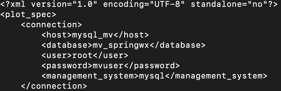
metviewer/plot_WIND_Z10.xml:
Change the database in the xml script to be "mv_springwx"
In addition, the other files can be modified based on the desired case specifics. For example, if you wish to change the variables being output in UPP, you will modify wrf_cntrl.parm (grib) or postcntrl.xml (grib2). If you are interested in changing variables, levels, or output types from MET, you will modify the MET configuration files under /met_config. More detailed information on the various components and their customization of WPS/WRF, UPP, and MET can be found in their respective User Guides:
With the scripts, namelists, and ancillary files ready for the new case, the next step is to retrieve the data for initial and boundary conditions, data assimilation, and verification.
Pulling data from AWS
Pulling data from AWSPulling data from Amazon S3 bucket
In this example, we will be retrieving 0.25° Global Forecast System (GFS) data from a publicly available Amazon Simple Storage Service (S3) bucket and storing it on our local filesystem, where it will be mounted for use in the Docker-space. The case is initialized at 00 UTC on 20210601 out to 24 hours in 3-hr increments.
To run the example case, first we need to set some variables and create directories that will be used for this specific example.
| tcsh | bash |
|---|---|
|
cd /home/ec2-user
setenv PROJ_DIR `pwd` setenv PROJ_VERSION 4.1.0
|
cd /home/ec2-user
export PROJ_DIR=`pwd` export PROJ_VERSION="4.1.0"
|
Then, you should set up the variables and directories for the experiment (spring_wx):
| tcsh | bash |
|---|---|
|
setenv CASE_DIR ${PROJ_DIR}/spring_wx
|
export CASE_DIR=${PROJ_DIR}/spring_wx
|
cd ${CASE_DIR}
mkdir -p wpsprd wrfprd gsiprd postprd pythonprd metprd metviewer/mysql
The GFS data needs to be downloaded into the appropriate directory, so we need to navigate to:
cd ${PROJ_DIR}/data/model_data/spring_wx
Next, run a script to pull GFS data for a specific initialization time (YYYYMMDDHH), maximum forecast length (HH), and increment of data (HH). For example:
If wget is not available on your system, an alternative is curl. You can, for example, modify the pull_aws_s3_gfs.ksh to have: curl -L -O
Run NWP initialization components (WPS, real.exe)
As with the provided canned cases, the first step in the NWP workflow will be to create the initial and boundary conditions for running the WRF model. This will be done using WPS and real.exe.
These commands are the same as the canned cases, with some case-specific updates to account for pointing to the appropriate scripts directory and name of the container.
SELECT THE APPROPRIATE CONTAINER INSTRUCTIONS FOR YOUR SYSTEM BELOW:
-v ${PROJ_DIR}/data/WPS_GEOG:/data/WPS_GEOG \
-v ${PROJ_DIR}/container-dtc-nwp/data:/data \
-v ${PROJ_DIR}/container-dtc-nwp/components/scripts/common:/home/scripts/common \
-v ${PROJ_DIR}/container-dtc-nwp/components/scripts/spring_wx:/home/scripts/case \
-v ${CASE_DIR}/wpsprd:/home/wpsprd \
--name run-springwx-wps dtcenter/wps_wrf:${PROJ_VERSION} /home/scripts/common/run_wps.ksh
-v ${PROJ_DIR}/data:/data \
-v ${PROJ_DIR}/container-dtc-nwp/components/scripts/common:/home/scripts/common \
-v ${PROJ_DIR}/container-dtc-nwp/components/scripts/spring_wx:/home/scripts/case \
-v ${CASE_DIR}/wpsprd:/home/wpsprd \
-v ${CASE_DIR}/wrfprd:/home/wrfprd \
--name run-springwx-real dtcenter/wps_wrf:${PROJ_VERSION} /home/scripts/common/run_real.ksh1
| tcsh | bash |
|---|---|
|
setenv TMPDIR ${CASE_DIR}/tmp
|
export TMPDIR=${CASE_DIR}/tmp
|
Updating Software Versions
Updating Software VersionsUpdating software component versions
Several components of the end-to-end WRF-based containerized system still undergo regular updates and public releases to the community (WPS, WRF, MET, METviewer), while others are frozen (GSI and UPP for WRF). If you would like to change the version of a component defined in the code base you have pulled from the NWP container project GitHub repository you will need to change the Dockerfile for that component in the source code.
Go to the wps_wrf directory:
Edit the Dockerfile to update the version number for WRF and WPS on lines 9 and 10. For example:
ENV WPS_VERSION 4.3
Once the version has been updated, follow the instructions for option #2 to build the dtcenter/wps_wrf image from scratch using the appropriate version number in the image name.
Go to the MET directory:
Edit the Dockerfile to update the version number for MET on line 8. For example:
Once the version has been updated, follow the instructions for option #2 to build the dtcenter/nwp-container-met image from scratch using the appropriate version number in the image name.
Go to the METviewer directory:
Edit the Dockerfile to update the version number for METviewer on line 8. The versions of METcalcpy (Python version of statistics calculation) and METplotpy (packages for plotting in METplus) may also be updated on lines 9 and 10. For example:
ENV METCALCPY_GIT_NAME v1.0.0
ENV METPLOTPY_GIT_NAME v1.0.0
Once the version has been updated, follow the instructions for option #2 to build the dtcenter/nwp-container-metviewer image from scratch using the appropriate version number in the image name.
NWP components
NWP componentsThe following sections provide examples of different customizations for the NWP software components. These examples are not exhaustive and are provided to give guidance for some common ways these components are modified and customized for new cases.
Changing WRF Namelist
Changing WRF NamelistChanging namelist options in WRF
Perhaps you'd like to rerun WRF with a different namelist option by changing a physics scheme. In this case, you'll want to rerun the WRF and all downstream components (i.e., UPP, Python graphics, MET, and METviewer), but you may not need to rerun the WPS, GSI, or Real components. In this example, we will demonstrate how to modify and rerun a container by modifying the namelist.input without deleting local output from a previous run.
Go to the scripts directory for the desired case:
Edit the namelist.input to making your desired modifications. For this example, we will change mp_physics from 4 (WSM5) to 8 (Thompson). **More information on how to set up and run WRF can be found on the Users' Page: http://www2.mmm.ucar.edu/wrf/users/
mp_physics = 8,
Rerun the WRF container using the local changes made to the namelist.input file and modifying the local WRF output directory (note: you can rename wrfprd whatever you choose):
Select the appropriate container instructions for your system below:
-v ${PROJ_DIR}/container-dtc-nwp/components/scripts/common:/home/scripts/common \
-v ${PROJ_DIR}/container-dtc-nwp/components/scripts/sandy_20121027:/home/scripts/case \
-v ${CASE_DIR}/wpsprd:/home/wpsprd -v ${CASE_DIR}/gsiprd:/home/gsiprd -v ${CASE_DIR}/wrfprd_mp6:/home/wrfprd \
--name run-sandy-wrf dtcenter/wps_wrf:${PROJ_VERSION} /home/scripts/common/run_wrf.ksh
Modify model domain
Modify model domainModifying the WRF model domain
This example demonstrates how to modify the domain for the Sandy case, but these procedures can be used as guidance for any other case as well.
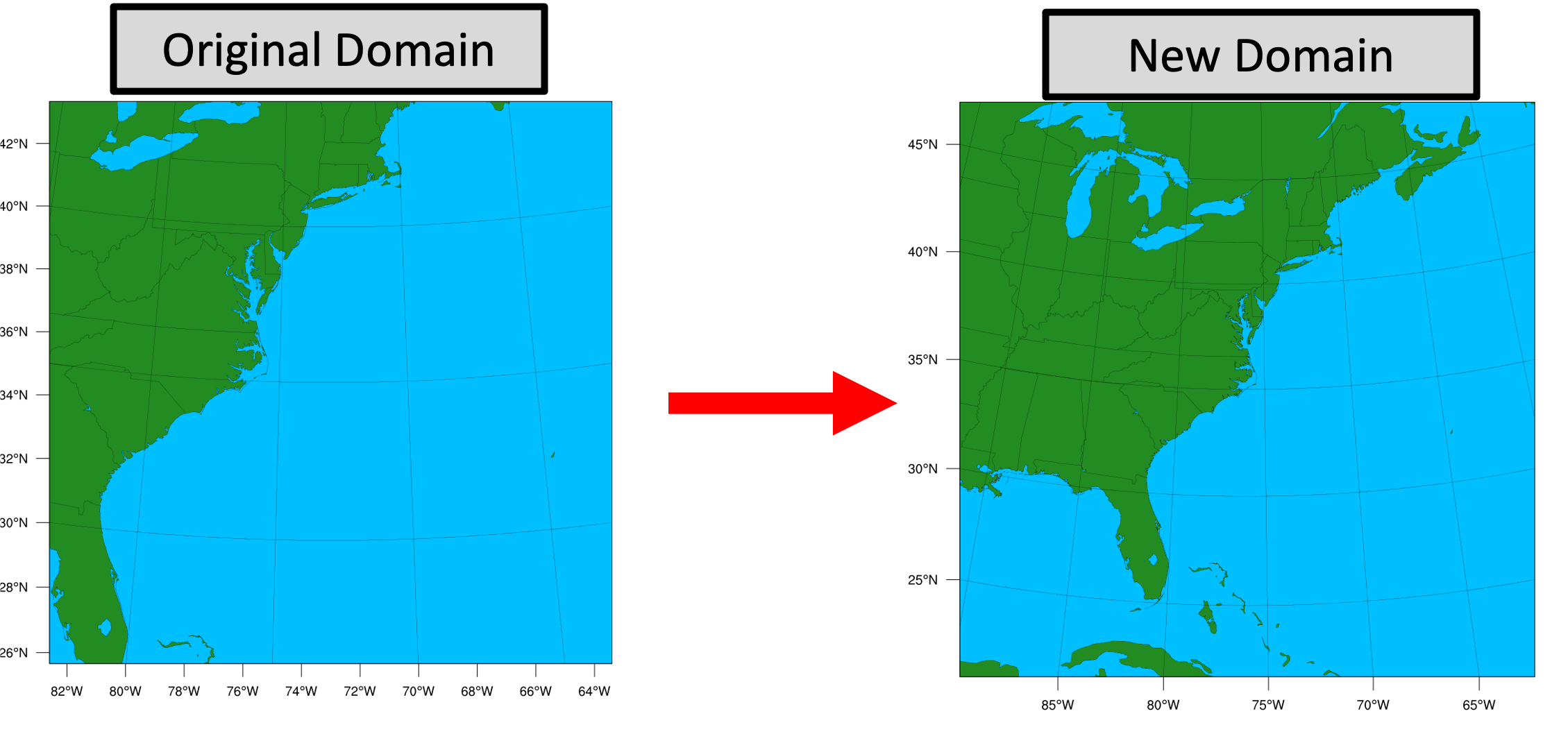
Changing the model domain requires modifying the WRF namelist.wps and namelist.input. For this example, let's say you want to make the original Sandy domain larger and shift it westward to include more land.
First, make sure you have created a new case directory so nothing is overwritten from the original run, and that your $CASE_DIR is properly set. See Setting Up a New Experiment
Next, modify the &geogrid section of the namelist.wps:
vi namelist.wps
Edits to &geogrid section of namelist.wps:
e_we: 50 --> 75 (line 15)
e_sn: 50 --> 75 (line 16)
ref_lon: -73. --> -76. (line 22)
stand_lon: -73.0 --> -76.0 (line 25)
The updated &geogrid section of the namelist.wps should look like this (with changes in bold):
parent_id = 1, 1,
parent_grid_ratio = 1, 3,
i_parent_start = 1, 31,
j_parent_start = 1, 17,
e_we = 75, 112,
e_sn = 75, 97,
geog_data_res = 'lowres', 'lowres',
dx = 40000,
dy = 40000,
map_proj = 'lambert',
ref_lat = 35.
ref_lon = -76.
truelat1 = 30.0,
truelat2 = 60.0,
stand_lon = -76.0,
geog_data_path = '/data/WPS_GEOG/',
opt_geogrid_tbl_path = '/comsoftware/wrf/WPS-4.1/geogrid',
/
The &domains section of the namelist.input file must also be updated to reflect these new domain parameters:
vi namelist.input
Edits to the &domains section of the namelist.input:
e_we: 50 --> 75 (line 38)
e_sn: 50 --> 75 (line 39)
time_step = 180,
time_step_fract_num = 0,
ime_step_fract_den = 1,
max_dom = 1,
e_we = 75, 112, 94,
e_sn = 75, 97, 91,
Now run the NWP components for your new case with the new domain.
SELECT THE APPROPRIATE CONTAINER INSTRUCTIONS FOR YOUR SYSTEM BELOW:
First run WPS:
Then run REAL:
Then run WRF:
-v ${PROJ_DIR}/container-dtc-nwp/components/scripts/common:/home/scripts/common \
-v ${PROJ_DIR}/container-dtc-nwp/components/scripts/sandy_20121027:/home/scripts/case \
-v ${CASE_DIR}/wpsprd:/home/wpsprd -v ${CASE_DIR}/gsiprd:/home/gsiprd -v ${CASE_DIR}/wrfprd:/home/wrfprd \
--name run-sandy-wrf dtcenter/wps_wrf:${PROJ_VERSION} /home/scripts/common/run_wrf.ksh
And continue running the remaining NWP components (i.e. UPP, MET, etc.)
First run WPS:
Then run REAL:
Then run WRF:
And continue running the remaining NWP components (i.e. UPP, MET, etc.)
Running WRF on multiple nodes with Singularity
Running WRF on multiple nodes with SingularityOne of the main advantages of Singularity is its broad support for HPC applications, specifically its lack of root privilege requirements and its support for scalable MPI on multi-node machines. This page will give an example of the procedure for running this tutorial's WPS/WRF Singularity container on multiple nodes on the NCAR Cheyenne supercomputer. The specifics of running on your particular machine of interest may be different, but you should be able to apply the lessons learned from this example to any HPC platform where Singularity is installed.
Step-by-step instructions
Load the singularity, gnu, and openmpi modules
module load gnu
module load openmpi
Set up experiment per usual (using snow case in this example)
git clone git@github.com:NCAR/container-dtc-nwp -b v${PROJ_VERSION}
mkdir data/ && cd data/
| tcsh | bash |
|---|---|
|
foreach f (/glade/p/ral/jntp/NWP_containers/*.tar.gz)
tar -xf "$f" end |
for f in /glade/p/ral/jntp/NWP_containers/*.tar.gz; do tar -xf "$f"; done
|
mkdir -p ${CASE_DIR} && cd ${CASE_DIR}
mkdir -p wpsprd wrfprd gsiprd postprd pythonprd metprd metviewer/mysql
export TMPDIR=${CASE_DIR}/tmp
mkdir -p ${TMPDIR}
Pull singularity image for wps_wrf from DockerHub
The Singularity containers used in this tutorial take advantage of the ability of the software to create Singularity containers from existing Docker images hosted on DockerHub. This allows the DTC team to support both of these technologies without the additional effort to maintain a separate set of Singularity recipe files. However, as mentioned on the WRF NWP Container page, the Docker containers in this tutorial contain some features (a so-called entrypoint script) to mitigate permissions issues seen with Docker on some platforms. Singularity on multi-node platforms does not work well with this entrypoint script, and because Singularity does not suffer from the same permissions issues as Docker, we have provided an alternate Docker container for use with Singularity to avoid these issues across multiple nodes:
Create a sandbox so the container is stored on disk rather than memory/temporary disk space
In the main tutorial, we create Singularity containers directly from the Singularity Image File (.sif). For multi-node Singularity, we will take advantage of an option known as "Sandbox" mode:
This creates a directory named "wps_wrf" that contains the entire directory structure of the singularity image; this is a way to interact with the Singularity container space from outside the container rather than having it locked away in the .sif file. You can use the ls command to view the contents of this directory, you will see it looks identical to the top-level directory structure of a typical linux install:
total 75
drwxr-xr-x 18 kavulich ral 4096 Feb 8 13:49 .
drwxrwxr-x 11 kavulich ral 4096 Feb 8 13:49 ..
-rw-r--r-- 1 kavulich ral 12114 Nov 12 2020 anaconda-post.log
lrwxrwxrwx 1 kavulich ral 7 Nov 12 2020 bin -> usr/bin
drwxr-xr-x 4 kavulich ral 4096 Feb 8 12:33 comsoftware
drwxr-xr-x 2 kavulich ral 4096 Feb 8 13:49 dev
lrwxrwxrwx 1 kavulich ral 36 Feb 8 13:42 environment -> .singularity.d/env/90-environment.sh
drwxr-xr-x 57 kavulich ral 16384 Feb 8 13:42 etc
lrwxrwxrwx 1 kavulich ral 27 Feb 8 13:42 .exec -> .singularity.d/actions/exec
drwxr-xr-x 4 kavulich ral 4096 Feb 8 12:52 home
lrwxrwxrwx 1 kavulich ral 7 Nov 12 2020 lib -> usr/lib
lrwxrwxrwx 1 kavulich ral 9 Nov 12 2020 lib64 -> usr/lib64
drwxr-xr-x 2 kavulich ral 4096 Apr 10 2018 media
drwxr-xr-x 2 kavulich ral 4096 Apr 10 2018 mnt
drwxr-xr-x 3 kavulich ral 4096 Dec 27 15:32 opt
drwxr-xr-x 2 kavulich ral 4096 Nov 12 2020 proc
dr-xr-x--- 5 kavulich ral 4096 Dec 27 16:00 root
drwxr-xr-x 13 kavulich ral 4096 Dec 27 16:20 run
lrwxrwxrwx 1 kavulich ral 26 Feb 8 13:42 .run -> .singularity.d/actions/run
lrwxrwxrwx 1 kavulich ral 8 Nov 12 2020 sbin -> usr/sbin
lrwxrwxrwx 1 kavulich ral 28 Feb 8 13:42 .shell -> .singularity.d/actions/shell
lrwxrwxrwx 1 kavulich ral 24 Feb 8 13:42 singularity -> .singularity.d/runscript
drwxr-xr-x 5 kavulich ral 4096 Feb 8 13:42 .singularity.d
drwxr-xr-x 2 kavulich ral 4096 Apr 10 2018 srv
drwxr-xr-x 2 kavulich ral 4096 Nov 12 2020 sys
lrwxrwxrwx 1 kavulich ral 27 Feb 8 13:42 .test -> .singularity.d/actions/test
drwxrwxrwt 7 kavulich ral 4096 Feb 8 12:53 tmp
drwxr-xr-x 13 kavulich ral 4096 Nov 12 2020 usr
drwxr-xr-x 18 kavulich ral 4096 Nov 12 2020 var
You can explore this directory to examine the contents of this container, but be cautious not to make any modifications that could cause problems later down the road!
Run WPS as usual
The command for running WPS is similar to that used in the main tutorial. Specifically, the fact that we are using a sandbox rather than creating a container straight from the singularity image file, requires a change to the run command. Note the bold part that is different from the original tutorial:
Prepare the wrfprd directory
Now this part is still a little hacky...but this will be cleaned up in future versions. Enter the wrfprd directory and manually link the met_em output files from WPS and rename them to the proper "nocolons" convention. Then, link in the contents of the WRF run directory containing the static input files and compiled executables from the container we created in a sandbox, and replace the default namelist with our case's custom namelist:
ln -sf ${CASE_DIR}/wps_wrf/comsoftware/wrf/WRF-4.3/run/* .
rm namelist.input
cp $PROJ_DIR/container-dtc-nwp/components/scripts/snow_20160123/namelist.input .
Finally, request as many cores/nodes as you want, reload the environment on compute nodes, and run!
qsub -V -I -l select=2:ncpus=36:mpiprocs=36 -q regular -l walltime=02:00:00 -A P48503002
ln -sf ${CASE_DIR}/wpsprd/met_em.* .
|
tcsh |
bash |
|---|---|
|
foreach f ( met_em.* )
setenv j `echo $f | sed s/\:/\_/g` mv $f $j end |
for f in met_em.*; do mv "$f" "$(echo "$f" | sed s/\:/\_/g)"; done
|
mpiexec -np 72 singularity run -u -B/glade:/glade ${CASE_DIR}/wps_wrf ./wrf.exe
The rest of the tutorial can be completed as normal.
Post Processing
Post ProcessingAdding a new output variable to UPP
Perhaps you would like to output a variable in WRF and UPP that is not part of the "out of the box" configuration provided with the tutorial cases. In this example, we will demonstrate how to modify the WRF namelist.input and UPP control files to output maximum updraft helicity. Note: This variable has already been added for the tutorial cases, but the steps provide a roadmap for other variables.
Go to the scripts directory for the desired case. In this example, we will be using the derecho case:
In order to output maximum updraft helicity, you will need to edit the WRF namelist.input by setting nwp_diagnostics = 1 under the time_control section in the namelist.input. See below for what this entry looks like:
run_days = 0,
run_hours = 24,
.
.
.
nwp_diagnostics = 1
/
For more information on the nwp_diagnostics package, please see the WRF documentation. Once the local changes to the namelist.input have been made, run WRF per the instructions in the tutorial. If the changes were successfully executed, you should see the UP_HELI_MAX variable in the WRF output.
Changes to the UPP control files are necessary to output maximum updraft helicity in the post-processed GRIB2 files. More extensive descriptions are provided in the UPP User's Guide, but the necessary steps will be briefly outlined below.
First, if you are not still in the scripts directory, navigate there:
The new variable needs to be added to the postcntrl.xml file, which is a file composed of a series of parameter blocks specifying the variables, fields, and levels. To add maximum helicity, add the following block (note: order in the file does not matter as long as the variables are within the </paramset> and </postxml> tags):
<shortname>MAX_UPHL_ON_SPEC_HGT_LVL_ABOVE_GRND_2-5km</shortname>
<pname>MXUPHL</pname>
<table_info>NCEP</table_info>
<scale>-3.0</scale>
</param>
Information on the specifics of populating the parameter blocks is available in the UPP User's Guide. Once the postcntrl.xml file is updated, additional control files need to be modified.
Due to software requirements, these changes need to be made using the UPP code directory that lives in the UPP container. To enter the container,
SELECT THE APPROPRIATE CONTAINER INSTRUCTIONS FOR YOUR SYSTEM BELOW:
To enter the Docker container, execute the following command:
-v ${PROJ_DIR}/container-dtc-nwp/components/scripts/derecho_20120629:/home/scripts/case \
--name run-derecho-upp dtcenter/upp:3.5.1 /bin/bash
All changes that need to be made will be under the UPP parm directory. First, the necessary control files need to be copied into the parm directory:
cp /home/scripts/case/post*xml .
An optional step to ensure the user-edited XML stylesheets (EMC_POST_CTRL_Scheme.xsd and EMC_POST_Avblflds_Scheme.xsd) are error free is to validate the postcntrl.xml and postavblflds.xml files. If the validation is successful, confirmation will be given (e.g., postcntrl.xml validates). Otherwise, it will return error messages. To run the optional validation step:
xmllint --noout --schema EMC_POST_Avblflds_Schema.xsd post_avblflds.xml
Once the XMLs are validated, the user will need to generate the flat file. Edit the makefile_comm to point to the full path of the parm directory in container space. The makefile_comm will call the perl program POSTXMLPreprocessor.pl to generate the flat file, postxconfig-NT_WRF.txt. Modify the makefile_comm to change the path of FLATFILEDIR and FLATFILENAME:
FLATFILENAME = postxconfig-NT_WRF.txt
To generate the flat file type:
make
If a new flat file is successfully generated, you will see a message "Flat file is new generated." In order to save the postxconfig-NT_WRF.txt file outside of the container, we need to move it to the directory in container space that is mounted to your local scripts directory. After that is complete, you can exit the container.
exit
After completing these steps, rerun the WRF and UPP steps as usual with Docker commands.
To enter the Singularity container, we can leverage the "sandbox" feature and make the changes locally. Execute the following command:
singularity build --sandbox upp_3.5.1 ${CASE_DIR}/upp_3.5.1.sif
This will create a directory called "upp_3.5.1" in your ${PROJ_DIR}. We can now go into that directory and leverage the already built UPP code to make the necessary changes.
cp ${PROJ_DIR}/dtc-nwp-container/components/scripts/derecho_20120629/post*xml .
An optional step to ensure the user-edited XML stylesheets (EMC_POST_CTRL_Scheme.xsd and EMC_POST_Avblflds_Scheme.xsd) are error free is to validate the postcntrl.xml and postavblflds.xml files. If the validation is successful, confirmation will be given (e.g., postcntrl.xml validates). Otherwise, it will return error messages. To run the optional validation step:
xmllint --noout --schema EMC_POST_Avblflds_Schema.xsd post_avblflds.xml
Once the XMLs are validated, the user will need to generate the flat file. Edit the makefile_comm to point to the full path of the parm directory in container space. The makefile_comm will call the perl program POSTXMLPreprocessor.pl to generate the flat file, postxconfig-NT_WRF.txt. Modify the makefile_comm to change the path of FLATFILEDIR and FLATFILENAME:
FLATFILENAME = postxconfig-NT_WRF.txt
To generate the flat file type:
make
If a new flat file is successfully generated, you will see a message "Flat file is new generated." We then want to make sure to copy this new postxconfig-NT_WRF.txt file to the local case scripts directory to ensure it is used.
Rerun WRF using the wps_wrf_3.5.1.sif as in the Derecho tutorial (note for this example we assume you're `pwd` is ${PROJ_DIR}:
Finally, run UPP using the "sandbox" Singularity container:
Some final notes on adding a new output variable with WRF and/or UPP:
-
In the official WRF release, maximum updraft helicity is already enabled to be output via the WRF Registry files. All that is needed to be available in the WRF output files is to modify the namelist.input by setting nwp_diagnostics = 1. If you need to modify the WRF Registry file, please contact us for assistance.
-
In the official UPP release, maximum updraft helicity is already a supported variable. While a large number of variables are supported, not all variables are written out. The original postcntrl.xml did not specify outputting maximum updraft helicity; therefore, modifications were made to add the variable to output. To add a new variable that is not available in UPP and to access a list of fields produced by UPP, please see the UPP User's Guide.
Graphics
GraphicsThis tutorial uses Python to visualize the post-processed model output. If users are familiar with Python, they may modify existing examples and/or create new plot types. As a note, while this tutorial supports plotting post-processed model output after running UPP, Python is also able to directly plot the NetCDF output from WRF (with numerous examples available online). Two customization options are provided below -- one for modifying the provided Python scripts and one for adding a new output variable to plot.
Modifying the provided Python script(s)
Users may modify existing script(s) by navigating to the /scripts/common directory and modifying the existing ALL_plot_allvars.py script (or the individual Python scripts). There are innumerable permutations for modifying the graphics scripts, based on user preferences, so one example will be chosen to show the workflow for modifying the plots. In this example, we will modify the ALL_plot_allvars.py script to change the contour levels used for plotting sea-level pressure.
Since the Hurricane Sandy case exceeds the current minimum value in the specified range, we will add 4 new contour levels. First, navigate to the Python plotting scripts directory:
vi ALL_plot_allvars.py
Edit the ALL_plot_allvars.py script to make the desired changes to the contour levels. For this example, we will be modifying line 466 from:
To extend the plotted values starting from 960 hPa:
After the new contour levels have been added, the plots can be generated using the same run command that is used for the supplied cases. Since we are interested in the impacts on the Hurricane Sandy plots, we will use the following run command:
-v ${PROJ_DIR}/container-dtc-nwp/components/scripts/common:/home/scripts/common \
-v ${PROJ_DIR}/container-dtc-nwp/components/scripts/sandy_20121027:/home/scripts/case \
-v ${PROJ_DIR}/data/shapefiles:/home/data/shapefiles \
-v ${CASE_DIR}/postprd:/home/postprd -v ${CASE_DIR}/pythonprd:/home/pythonprd \
--name run-sandy-python dtcenter/python:${PROJ_VERSION} /home/scripts/common/run_python.ksh
Adding a new plot type
In addition to modifying the ALL_plot_allvars.py for the current supported variables, users may want to add new variables to plot. The Python scripts use the pygrib module to read GRIB2 files. In order to determine what variables are available in the post-processed files and their names as used by pygrib, a simple script, read_grib.py, under the /scripts/common directory, is provided to print the variable names from the post-processed files. For this example, we will plot a new variable, wind at 850 hPa. This will require us to run the read_grib.py script to determine the required variable name. In order to run read_grib.py, we are assuming the user does not have access to Python and the necessary modules, so we will use the Python container. To enter the container, execute the following command:
-v ${PROJ_DIR}/container-dtc-nwp/components/scripts/common:/home/scripts/common \
-v ${PROJ_DIR}/container-dtc-nwp/components/scripts/sandy_20121027:/home/scripts/case \
-v ${PROJ_DIR}/data/shapefiles:/home/data/shapefiles \
-v ${CASE_DIR}/postprd:/home/postprd -v ${CASE_DIR}/pythonprd:/home/pythonprd \
--name run-sandy-python dtcenter/python:${PROJ_VERSION} /bin/bash
Once "in" the container, navigate to the location of the read_grib.py script and open the script:
vi read_grib.py
This script reads a GRIB2 file output from UPP, so this step does require that the UPP step has already been run. To execute the script:
For the standard output from the Hurricane Sandy case, here is the output from executing the script:
After perusing the output, you can see that the precipitable water variable is called 'Precipitable water.' To add the new variable to the ALL_plot_allvars.py script, it is easiest to open the script and copy the code for plotting a pre-existing variable (e.g., composite reflectivity) and modify the code for precipitable water:
In the unmodified ALL_plot_allvars.py script, copy lines 367-368 for reading in composite reflectivity, paste right below, and change the variable to be for precipitable water, where 'Precipitable water' is variable name obtained from the output of the read_grib.py:
![]()
Next, we will add a new code block for plotting precipitable water, based on copying, pasting, and modifying from the composite reflectivity block above it (lines 731-760 in the unmodified code):
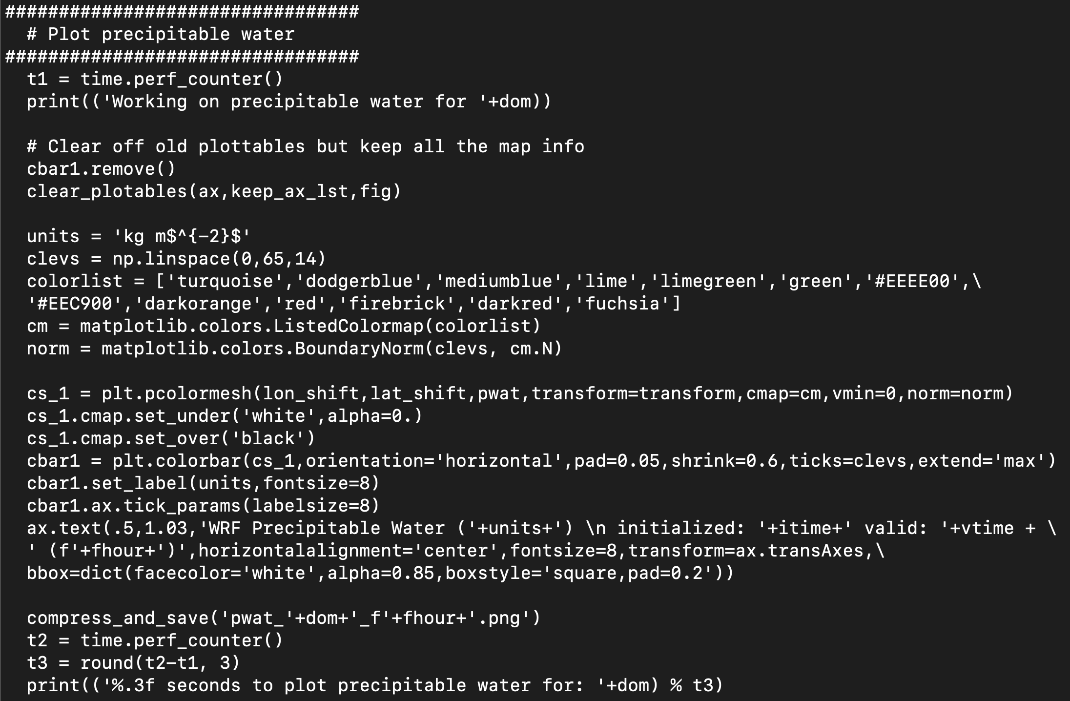
Note: This is a simple example of creating a new plot from the UPP output. Python has a multiple of customization options, with changes to colorbars, color maps, etc. For further customization, please refer to online resources.
To generate the new plot type, point to the scripts in the local scripts directory, run the dtcenter/python container to create graphics in docker-space and map the images into the local pythonprd directory:
-v ${PROJ_DIR}/container-dtc-nwp/components/scripts/common:/home/scripts/common \
-v ${PROJ_DIR}/container-dtc-nwp/components/scripts/sandy_20121027:/home/scripts/case \
-v ${PROJ_DIR}/data/shapefiles:/home/data/shapefiles \
-v ${CASE_DIR}/postprd:/home/postprd -v ${CASE_DIR}/pythonprd:/home/pythonprd \
--name run-sandy-python dtcenter/python:${PROJ_VERSION} /home/scripts/common/run_python.ksh
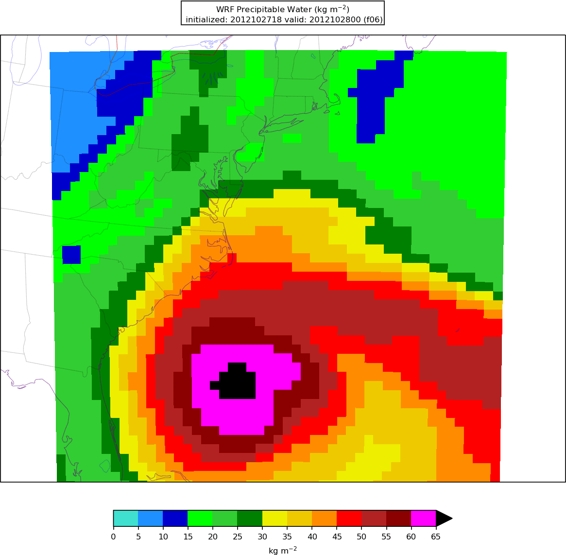
After Python has been run, the plain image output files will appear in the local pythonprd directory.
Here is an example of resulting plot of the precipitable water:
Verification
VerificationThe Model Evaluation Tools (MET) package includes many tools for forecast verification. More detailed information about MET can be found at the MET User's Page. The following MET tools are run by the /scripts/common/run_met.ksh shell script:
- PB2NC : pre-processes point observations from PREPBUFR files
- Point-Stat : verifies model output against point observations
- PCP-Combine : modifies precipitation accumulation intervals
- Grid-Stat : verifies model output against gridded analyses
The processing logic for these tools is specified by ASCII configuration files. Take a look at one of these configuration files:
- ${PROJ_DIR}/container-dtc-nwp/components/scripts/sandy_20121027/met_config/PointStatConfig_ADPSFC
Here you could add to or subtract from the list of variables to be verified. You could change the matching observation time window, modify the interpolation method, choose different output statistic line types, or make any number of other modifications. After modifying the MET configuration, rerunning the Docker run command for the verification component will recreate the MET output.
Database and display
Database and displayThe METviewer database and display system provides a flexible and interactive interface to ingest and visualize the statistical output of MET. In this tutorial, we loaded the MET outputs for each of the 3 supported case into separate databases named mv_derecho, mv_sandy, and mv_snow, which required running METviewer separately for each case by pointing to the specific ${CASE_DIR} directory. While sometimes it is desirable for each case to have its own database within a single METviewer instance, sometimes it is advantageous to load MET output from multiple cases into the same METviewer instance. For example, if a user had multiple WRF configurations they were running over one case, and they wanted to track the performance of the different configurations, they could load both case outputs into METviewer and analyze them together. The customization example below demonstrates how to load MET output from multiple cases into a METviewer database.
Load MET output from multiple cases into a METviewer database
In this example, we will execute a series of three steps: 1) reorganize the MET output from multiple cases to live under a new, top-level directory, 2) launch the METviewer container, using a modified Docker compose YML file, and 3) execute a modified METviewer load script to load the data into the desired database. For example purposes, we will have two cases: sandy (supplied, unmodified sandy case from the tutorial) and sandy_mp8 (modified sandy case to use Thompson microphysics, option 8); these instructions will only focus on the METviewer steps, assuming the cases have been run through the step to execute MET and create verification output.
Step 1: Reorganize the MET output
In order to load MET output from multiple cases in a METviewer database, the output must be rearranged from its original directory structure (e.g., $PROJ_DIR/sandy) to live under a new, top-level cases directory (e.g., $PROJ_DIR/cases/sandy). In addition, a new, shared metviewer/mysql directory must also be created.
mkdir -p $PROJ_DIR/metviewer/mysql
Once the directories are created, the MET output needs to be copied from the original location to the new location.
cp -r $PROJ_DIR/sandy_mp8/metprd/* $PROJ_DIR/cases/sandy_mp8
Step 2: Launch the METviewer container
In order to visualize the MET output from multiple cases using the METviewer database and display system, you first need to launch the METviewer container. These modified YML files differ from the original files used in the supplied cases by modifying the volume mounts to no longer be case-specific (i.e., use $CASE_DIR).
| FOR NON-AWS: | FOR AWS: |
|---|---|
|
|
|
Step 3: Load MET output into the database(s)
The MET output then needs to be loaded into the MySQL database for querying and plotting by METviewer by executing the load script (metv_load_cases.ksh), which requires three command line arguments: 1) name of database to load MET output (e.g., mv_cases), 2) path in Docker space where the case data will be mapped, which will be /data/{name of case directory used in Step 1}, and 3) whether you want a new database to load MET output into (YES) or load MET output into a pre-existing database (NO). In this example, where we have sandy and sandy_mp8 output, the following commands would be issued:
docker exec -it metviewer /scripts/common/metv_load_cases.ksh mv_cases /data/sandy_mp8 NO
The METviewer GUI can then be accessed with the following URL copied and pasted into your web browser:
Note, if you are running on AWS, run the following commands to reconfigure METviewer with your current IP address and restart the web service:
|
docker exec -it metviewer /bin/bash
/scripts/common/reset_metv_url.ksh exit |
The METviewer GUI can then be accessed with the following URL copied and pasted into your web browser (where IPV4_public_IP is your IPV4Public IP from the AWS “Active Instances” web page):
http://IPV4_public_IP/metviewer/metviewer1.jsp
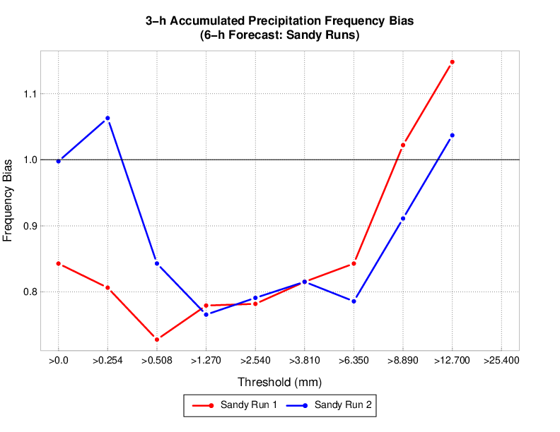
These commands would load sandy and sandy_mp8 MET output into the mv_cases database. An example METviewer plot using sandy sandy_mp8 MET output is shown below (click here for XML used to create the plot).
Modifying a container image
Modifying a container imageCurrently, procedures for this feature are only provided for Docker containers.
There may be a desire to make a change within a Docker container image and then use that updated image in an experiment. For example, you could make changes to the source code of a component, or modify default tables of a software component, etc. You The command docker commit allows one to save changes made within an existing container to a new image for future use.
In this example, we'll modify the wps_wrf container. Assuming you already have the wps_wrf:4.0.0 image pulled from Dockerhub (4.0.0. being the previously set ${PROJ_VERSION} variable), you should see your images following the docker images command. For example:
dtcenter/wps_wrf 4.0.0 3d78d8d63aec 2 months ago 3.81GB
We will deploy the container similar to running a component in our example cases, however with a few key difference. First, we'll omit the "--rm" option from the command so that when we exit the container it is not removed from our local list of containers and the changes persist in a local container. For simplicity, we'll also omit the mounting of local directories. Finally, we'll substitute our typical run command from a provided script to a simple /bin/bash. This allows us to enter the container in a shell environment to make changes and test any modifications.
[comuser@d829d8d812d6 wrf]$
Note the change in command prompt to something similar to: [comuser@d829d8d812d6 wrf]$, highlighting that you are now inside the container, and not on your local machine space. Do an "ls" to list what's in this container:
WPS-4.3 WRF WRF-4.3
Inside the container, you can now make any edits you want. You could make an edit to the WRF or WPS source code and recompile the code, or your make edits to predefined tables. For the purposes of illustrating the general concept of docker commit, we'll just add a text file in the container so we can see how to make it persist in a new image.
ls
Now exit the container.
You are now back on your local command line. List your containers to find the name of the container that you just modified and exited:
d829d8d812d6 dtcenter/wps_wrf:4.0.0 "/usr/local/bin/entr…" 33 seconds ago Exited (0) 20 seconds ago sweet_moser
Note the container d829d8d812d6 that we just exited. This is the container name id that we'll use to make a new image. Use docker commit to create a new image from that modified container. The general command is:
docker commit CONTAINER_ID_NAME NEW_IMAGE_NAME
So in this example:
Execute a docker images command to list your images and see the new image name.
wps_wrf_testfile latest f490d863a392 3 seconds ago 3.81GB
dtcenter/wps_wrf 4.0.0 3d78d8d63aec 2 months ago 3.81GB
You can deploy this new image and enter the container via a shell /bin/bash command to confirm this new image has your changes, e.g.:
useradd: user 'user' already exists
[comuser@05e6fb4618dd wrf]$
In the container, now do a "ls" to list the contents and see the test file.
Exit the container.
Once you have this new image, you can use it locally as needed. You could also push it to a Dockerhub repository where it will persist beyond your local machine and enable you to use docker pull commands and share the new image if needed.