Session 3: Ensemble and PQPF
Session 3: Ensemble and PQPF
METplus Practical Session 3
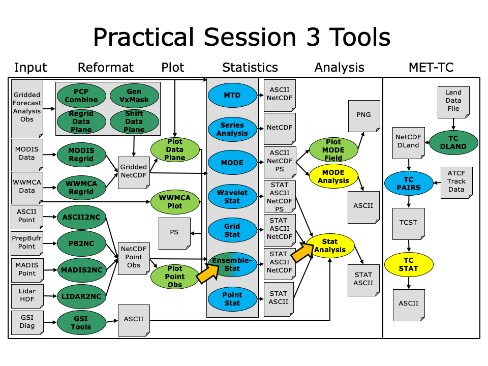
During this practical session, you will run the tools indicated below:
You may navigate through this tutorial by following the links at the bottom of each page or by using the menu navigation.
Since you already set up your runtime enviroment in Session 1, you should be ready to go! To be sure, run through the following instructions to check that your environment is set correctly.
Prerequisites: Verify Environment is Set Correctly
Before running these instructions, you will need to ensure that you have a few environment variables set up correctly. If they are not set correctly, these instructions will not work properly.
- Check that you have METPLUS_TUTORIAL_DIR set correctly:
ls ${METPLUS_TUTORIAL_DIR}
If you don't see a path in your user directory output to the screen, set this environment variable in your user profile before continuing.
- Check that you have METPLUS_BUILD_BASE, MET_BUILD_BASE, and METPLUS_DATA set correctly:
echo ${MET_BUILD_BASE}
echo ${METPLUS_DATA}
ls ${METPLUS_BUILD_BASE}
ls ${MET_BUILD_BASE}
ls ${METPLUS_DATA}
If any of these variables are not set, please set them. They will be referenced throughout the tutorial.
MET_BUILD_BASE is the full path to the MET installation (/path/to/met-X.Y)
METPLUS_DATA is the location of the sample test data directory
- Check that you have loaded the MET module correctly:
You should see the usage statement for Point-Stat. The version number listed should correspond to the version listed in MET_BUILD_BASE. If it does not, you will need to either reload the met module, or add ${MET_BUILD_BASE}/bin to your PATH.
- Check that METPLUS_PARM_BASE was set correctly.
ls ${METPLUS_PARM_BASE}
If you don't see the full path to your METplus/parm directory under the tutorial directory, please set it. See the instructions in Session 1 for more information.
- Check that the correct version of master_metplus.py is in your PATH:
If you don't see the full path to script from the shared installation, please set it. It should look the same as the output from this command:
ls ${METPLUS_BUILD_BASE}/ush/master_metplus.py
See the instructions in Session 1 for more information.
You are now ready to move on to the next section.
MET Tool: Ensemble-Stat
MET Tool: Ensemble-Stat
Ensemble-Stat Tool: General
Ensemble-Stat Functionality
The Ensemble-Stat tool may be used to derive several summary fields, such as the ensemble mean, spread, and relative frequencies of events (i.e. similar to a probability). The summary fields produced by Ensemble-Stat may then be verified using the other MET statistics tools. Ensemble-Stat may also be used to verify the ensemble directly by comparing it to gridded and/or point observations. Statistics are then derived using those observations, such as rank histograms and the continuous ranked probability score.
Ensemble-Stat Usage
View the usage statement for Ensemble-Stat by simply typing the following:
At a minimum, the input gridded ensemble files and the configuration config_file must be passed in on the command line. You can specify the list of ensemble files to be used either as a count of the number of ensemble members followed by the file name for each (n_ens ens_fil e_1 ... ens_file_n) or as an ASCII file containing the names of the ensemble files to be used (ens_file_list). Choose whichever way is most convenient for you. The optional -grid_obs and -point_obs command line options may be used to specify gridde d and/or point observations to be used for computing rank histograms and other ensemble statistics.
As with the other MET statistics tools, all ensemble data and gridded verifying observations must be interpolated to a common grid prior to processing. This may be done using the automated regrid feature in the Ensemble-Stat configuration file or by running copygb and/or wgrib2 first.
Ensemble-Stat Tool: Configure
Ensemble-Stat Tool: Configure
Start by making an output directory for Ensemble-Stat and changing directories:
cd ${METPLUS_TUTORIAL_DIR}/output/met_output/ensemble_stat
The behavior of Ensemble-Stat is controlled by the contents of the configuration file passed to it on the command line. The default Ensemble-Stat configuration file may be found in the data/config/EnsembleStatConfig_default file. The configurations used by the test script may be found in the scripts/config/EnsembleStatConfig* files. Prior to modifying the configuration file, users are advised to make a copy of the default:
Open up the EnsembleStatConfig_tutorial file for editing with your preferred text editor.
The configurable items for Ensemble-Stat are broken out into two sections. The first section specifies how the ensemble should be processed to derive summary fields, such as the ensemble mean and spread. The second section specifies how the ensemble should be verified directly, such as the computation of rank histograms and spread/skill. The configurable items include specifications for the following:
- Section 1: Ensemble Processing (ens dictionary)
- The ensemble fields to be summarized at the specified vertical level or accumulation interval.
- The threshold values to be applied in computing ensemble relative frequencies (e.g. the percent of ensemble members exceeding some threshold at each point).
- Thresholds to specify how many of the ensemble members must actually be present with valid data.
- Section 2: Verification (fcst and obs dictionaries)
- The forecast and observation fields to be verified at the specified vertical level or accumulation interval.
- The matching time window for point observations.
- The type of point observations to be matched to the forecasts.
- The areas over which to aggregate statistics - as predefined grids or configurable lat/lon polylines.
- The interpolation or smoothing methods to be used.
You may find a complete description of the configurable items in section 9.3.2 of the MET User's Guide. Please take some time to review them.
For this tutorial, we'll configure Ensemble-Stat to summarize and verify 24-hour accumulated precipitation. While we'll run Ensemble-Stat on a single field, please note that it may be configured to operate on multiple fields. The ensemble we're verifying consists of 6 members defined over the west coast of the United States. Edit the EnsembleStatConfig_tutorial file as follows:
- In the ens dictionary, set
field = [
{
name = "APCP";
level = [ "A24" ];
cat_thresh = [ >0, >=5.0, >=10.0 ];
}
];To read 24-hour accumulated precipitation from the input GRIB files and compute ensemble relative frequencies for the thresolds listed.
- In the fcst dictionary, set
field = [
{
name = "APCP";
level = [ "A24" ];
}
];To also verify the 24-hour accumulated precipitation fields.
-
In the fcst dictionary, set:
message_type = [ "ADPSFC" ];To verify against surface observations.
- In the mask dictionary, set:
grid = [ "FULL" ];To accumulate statistics over the full model domain.
- In the mask dictionary, set
poly = [ "MET_BASE/poly/NWC.poly",
"MET_BASE/poly/SWC.poly" ];To also verify over the northwest coast (NWC) and southwest coast (SWC) subregions.
- Set:
output_flag = {
ecnt = BOTH;
rhist = BOTH;
phist = BOTH;
orank = BOTH;
ssvar = BOTH;
relp = BOTH;
}To compute continuous ensemble statistics (ECNT), ranked histogram (RHIST), probability integral transform histogram (PHIST), observation ranks (ORANK), spread-skill variance (SSVAR), and relative position (RELP).
Save and close this file.
Ensemble-Stat Tool: Run
Ensemble-Stat Tool: Run
Next, run Ensemble-Stat on the command line using the following command, using wildcards to list the 6 input ensemble member files:
6 ${METPLUS_DATA}/met_test/data/sample_fcst/2009123112/*gep*/d01_2009123112_02400.grib \
EnsembleStatConfig_tutorial \
-grid_obs ${METPLUS_DATA}/met_test/data/sample_obs/ST4/ST4.2010010112.24h \
-point_obs ${METPLUS_DATA}/met_test/out/ascii2nc/precip24_2010010112.nc \
-outdir . \
-v 2
 The command above uses the ASCII2NC output of that was generated by make test when MET was compiled.
Ensemble-Stat is now performing the tasks we requested in the configuration file. Note that we've passed the input ensemble data directly on the command line by specifying the number of ensemble members (6) followed by their names using wildcards. We've also specified one gridded StageIV analysis field (-grid_obs) and one file containing point rain gauge observations (-point_obs) to be used in computing rank histograms. This tool should run pretty quickly.
When Ensemble-Stat is finished, it will have created 9 output files in the current directory: 6 ASCII statistics files (.stat, _ecnt.txt, _rhist.txt, _phist.txt, _orank.txt, _ssvar.txt , and _relp.txt ) , a NetCDF ensemble file (_ens.nc), and a NetCDF matched pairs file (_orank.nc).
Ensemble-Stat Tool: Output
Ensemble-Stat Tool: Output
The _ens.nc output from Ensemble-Stat is a NetCDF file containing the derived ensemble fields, one or more ASCII files containing statistics summarizing the verification performed, and a NetCDF file containing the gridded matched pairs.
All of the line types are written to the file ending in .stat. The Ensemble-Stat tool currently writes six output line types, ECNT, RHIST, PHIST, RELP, SSVAR, and ORANK.
- The ECNT line type contains contains continuous ensemble statistics such as spread and skill. Ensemble-Stat uses assumed observation errors to compute both perturbed and unperturbed versions of these statistics. Statistics to which observation error have been applied can be found in columns which include the _OERR (for observation error) suffix.
- The RHIST line type contains counts for a ranked histogram. This ranks each observation value relative to ensemble member values. Ideally, observation values would fall equally across all available ranks, yiedling a flat rank histogram. In practice, ensembles are often under-(U shape) or over-(inverted U shape) dispersive. In the event of ties, ranks are randomly assigned.
- The PHIST line type contains counts for a probability integral transform histogram. This scales the observation ranks to a range of values between 0 and 1 and allows ensembles of different size to be compared. Similiary, when ensemble members drop out, RHIST lines cannot be aggregated together but PHIST lines can.
- The RELP line is the relative position, which indicates how often each ensemble member's value was closest to the observation's value. In the event of ties, credit is divided equally among the tied members.
- The ORANK line type is similar to the matched pair (MPR) output of Point-Stat. For each point observation value, one ORANK line is written out containing the observation value, it's rank, and the corresponding ensemble values for that point. When verifying against a griddedanalysis, the ranks can be written to the NetCDF output file.
- The SSVAR line contains binned spread/skill information. For each observation location, the ensemble variance is computed at that point. Those variance values are binned based on the ens_ssvar_bin_size configuration setting. The skill is deteremined by comparing the ensemble mean value to the observation value. One SSVAR line is written for each bin summarizing the all the observation/ensemble mean pairs that it contains.
The STAT file contains all the ASCII output while the _ecnt.txt, _rhist.txt, _phist.txt, _orank.txt, _ssvar.txt, and _relp.txtfiles contain the same data but sorted by line type. Since so much data can be written for the ORANK line type, we recommend disabling the output of the optional text file using the output_flag parameter in the configuration file.
Since the lines of data in these ASCII file are so long, we strongly recommend configuring your text editor to NOT use dynamic word wrapping. The files will be much easier to read that way.
Open up the ensemble_stat_20100101_120000V_rhist.txt RHIST file using the text editor of your choice and note the following:
- There are 6 lines in this output file resulting from using 3 verification regions in the VX_MASK column (FULL, NWC, and SWC) and two observations datasets in the OBTYPE column (ADPSFC point observations and gridded observations).
- Each line contains columns for the observations ranks (RANK_#) and a handful of ensemble statistics (CRPS, CRPSS, IGN, and SPREAD).
- There is output for 7 ranks - since we verified a 6-member ensemble, there are 7 possible ranks the observation values could attain.
Close this file, and open up the ensemble_stat_20100101_120000V_phist.txt PHIST file, and note the following:
- There are 5 lines in this output file resulting from using 3 verification regions (FULL, NWC, and SWC) and two observations datasets (ADPSFC point observations and gridded observations), where the ADPSFC point observations for the SWC region were all zeros for which the probability integral transform is not defined.
- Each line contains columns for the BIN_SIZE and counts for each bin. The bin size is set in the configuration file using the ens_phist_bin_size field. In this case, it was set to .05, therefore creating 20 bins (1/ens_phist_bin_size).
Close this file, and open up the ensemble_stat_20100101_120000V_orank.txt ORANK file, and note the following:
- This file contains 1866 lines, 1 line for each observation value falling inside each verification region (VX_MASK).
- Each line contains 44 columns... header information, the observation location and value, it's rank, and the 6 values for the ensemble members at that point.
- When there are ties, Ensemble-Stat randomly assigns a rank from all the possible choices. This can be seen in the SWC masking region where all of the observed values are 0 and the ensemble forecasts are 0 as well. Ensemble-Stat randomly assigns a rank between 1 and 7.
Close this file, and use the ncview utility to view the NetCDF ensemble fields file:
This file contains variables for the following:
- Ensemble Mean
- Ensemble Standard Deviation
- Ensemble Mean minus 1 Standard Deviation
- Ensemble Mean plus 1 Standard Deviation
- Ensemble Minimum
- Ensemble Maximum
- Ensemble Range
- Ensemble Valid Data Count
- Ensemble Relative Frequency (for 3 thresholds)
The output of any of these summary fields may be disabled using the output_flag parameter in the configuration file.
Use the ncview utility to view the NetCDF gridded observation rank file:
This file is only created when you've verified using gridded observations and have requested its output using the output_flagparameter in the configuration file. Click through the variables in this file. Note that for each of the three verification areas (FULL, NWC, and SWC) this file contains 4 variables:
- The gridded observation value
- The observation rank
- The probability integral transform
- The ensemble valid data count
In ncview, the random assignment of tied ranks is evident in areas of zero precipitation.
Close this file.
Feel free to explore using this dataset. Some options to try are:
- Try setting skip_const = TRUE; in the config file to discard points where all ensemble members and the observaiton are tied (i.e. zero precip).
- Try setting obs_thresh = [ >0.01 ]; in the config file to only consider points where the observation meets this threshold. How does this differ from the using skip_const?
- Use wgrib to inventory the input files and add additional entries to the ens.field list. Can you process 10-meter U and V wind?
MET Tool: Stat-Analysis
MET Tool: Stat-Analysis
Stat-Analysis Tool: General
Stat-Analysis Functionality
The Stat-Analysis tool reads the ASCII output files from the Point-Stat, Grid-Stat, Wavelet-Stat, and Ensemble-Stat tools. It provides a way to filter their STAT data and summarize the statistical information they contain. If you pass it the name of a directory, Stat-Analysis searches that directory recursively and reads any .stat files it finds. Alternatively, if you pass it an explicit file name, it'll read the contents of the file regardless of the suffix, enabling it to the the optional _LINE_TYPE.txt files. Stat-Analysis runs one or more analysis jobs on the input data. It can be run by specifying a single analysis job on the command line or multiple analysis jobs using a configuration file. The analysis job types are summarized below:
- The filter job simply filters out lines from one or more STAT files that meet the filtering options specified.
- The summary job operates on one column of data from a single STAT line type. It produces summary information for that column of data: mean, standard deviation, min, max, and the 10th, 25th, 50th, 75th, and 90th percentiles.
- The aggregate job aggregates STAT data across multiple time steps or masking regions. For example, it can be used to sum contingency table data or partial sums across multiple lines of data. The -line_type argument specifies the line type to be summed.
- The aggregate_stat job also aggregates STAT data, like the aggregate job above, but then derives statistics from that aggregated STAT data. For example, it can be used to sum contingency table data and then write out a line of the corresponding contingency table statistics. The -line_type and -out_line_type arguments are used to specify the conversion type.
- The ss_index job computes a skill-score index, of which the GO Index (go_index) is a special case. The GO Index is a performance metric used primarily by the United States Air Force.
- The ramp job processes a time series of data and identifies rapid changes in the forecast and observation values. These forecast and observed ramp events are used populate a 2x2 contingency table from which categorical statistics are derived.
Stat-Analysis Usage
View the usage statement for Stat-Analysis by simply typing the following:
| Usage: stat_analysis | ||
| -lookin path | Space-separated list of input paths where each is a _TYPE.txt file, STAT file, or directory which should be searched recursively for STAT files. Allows the use of wildcards (required). | |
| [-out filename] | Output path or specific filename to which output should be written rather than the screen (optional). | |
| [-tmp_dir path] | Override the default temporary directory to be used (optional). | |
| [-log file] | Outputs log messages to the specified file | |
| [-v level] | Level of logging | |
| [-config config_file] | [JOB COMMAND LINE] (Note: "|" means "or") | ||
| [-config config_file] | STATAnalysis config file containing Stat-Analysis jobs to be run. | |
| [JOB COMMAND LINE] | All the arguments necessary to perform a single Stat-Analysis job. See the MET Users Guide for complete description of options. |
At a minimum, you must specify at least one directory or file in which to find STAT data (using the -lookin path command line option) and either a configuration file (using the -config config_file command line option) or a job command on the command line.
Stat-Analysis Tool: Configure
Stat-Analysis Tool: Configure
Stat-Analysis Tool: Configure
Start by making an output directory for Stat-Analysis and changing directories:
cd ${METPLUS_TUTORIAL_DIR}/output/met_output/stat_analysis
The behavior of Stat-Analysis is controlled by the contents of the configuration file or the job command passed to it on the command line. The default Stat-Analysis configuration may be found in the data/config/StatAnalysisConfig_default file. Let's start with a configuration file that's packaged with the met-8.0 test scripts:
Open up the STATAnalysisConfig_tutorial file for editing with your preferred text editor.
You will see that most options are left blank, so the tool will use whatever it finds or whatever is specified in the command or job line. If you go down to the jobs[]section you will see a list of the jobs run for the test scripts. Remove those existing jobs and add the following 2 analysis jobs:
"-job aggregate -line_type CTC -fcst_thresh >273.0 -vx_mask FULL -interp_mthd NEAREST",
"-job aggregate_stat -line_type CTC -out_line_type CTS -fcst_thresh >273.0 -vx_mask FULL -interp_mthd NEAREST"
];
The first job listed above will select out only the contingency table count lines (CTC) where the threshold applied is >273.0 over the FULL masking region. This should result in 2 lines, one for pressure levels P850-500 and one for pressure P1050-850. So this job will be aggregating contingency table counts across vertical levels.
The second job listed above will perform the same aggregation as the first. However, it'll dump out the corresponding contingency table statistics derived from the aggregated counts.
Stat-Analysis Tool: Run on Point-Stat output
Stat-Analysis Tool: Run on Point-Stat output
Stat-Analysis Tool: Run on Point-Stat output
Now, run Stat-Analysis on the command line using the following command:
-config STATAnalysisConfig_tutorial \
-lookin ../point_stat \
-v 2
The output for these two jobs are printed to the screen. Try redirecting their output to a file by adding the -out command line argument:
-config STATAnalysisConfig_tutorial \
-lookin ../point_stat \
-v 2 \
-out aggr_ctc_lines.out
The output was written to aggr_ctc_lines.out. We'll look at this file in the next section.
Next, try running the first job again, but entirely on the command line without a configuration file:
-lookin ../point_stat \
-v 2 \
-job aggregate \
-line_type CTC \
-fcst_thresh ">273.0" \
-vx_mask FULL \
-interp_mthd NEAREST
Note that we had to put double quotes (") around the forecast theshold string for this to work.
Next, run the same command but add the -dump_row command line option. This will redirect all of the STAT lines used by the job to a file. Also, add the -out_stat command line option. This will write a full STAT output file, including the 22 header columns:
-lookin ../point_stat \
-v 2 \
-job aggregate \
-line_type CTC \
-fcst_thresh ">273.0" \
-vx_mask FULL \
-interp_mthd NEAREST \
-dump_row aggr_ctc_job.stat \
-out_stat aggr_ctc_job_out.stat
Open up the file aggr_ctc_job.stat to see the 2 STAT lines used by this job.
Open up the file aggr_ctc_job_out.stat to see the 1 output STAT line. Notice that the FCST_LEV and OBS_LEV columns contain the input strings concatenated together.
Try re-running this job using -set_hdr FCST_LEV P1050-500 and -set_hdr OBS_LEV P1050-500. How does that affect the output?
The use of the -dump_row option is highly recommended to ensure that your analysis jobs run on the exact set of data that you intended. It's easy to make mistakes here!
Stat-Analysis Tool: Output
Stat-Analysis Tool: Output
Stat-Analysis Tool: Output
On the previous page, we generated the output file aggr_ctc_lines.out by using the -out command line argument. Open that file using the text editor of your choice, and be sure to turn word-wrapping off.
This file contains the output for the two jobs we ran through the configuration file. The output for each job consists of 3 lines as follows:
- The JOB_LIST line contains the job filtering parameters applied for this job.
- The COL_NAME line contains the column names for the data to follow in the next line.
- The third line consists of the line type generated (CTC and CTS in this case) followed by the values computed for that line type.
Next, try running the Stat-Analysis tool on the output file ../point_stat/point_stat_run2_360000L_20070331_120000V.stat. Start by running the following job:
-lookin ../point_stat/point_stat_run2_360000L_20070331_120000V.stat \
-v 2 \
-job aggregate \
-fcst_var TMP \
-fcst_lev Z2 \
-vx_mask EAST -vx_mask WEST \
-interp_pnts 1 \
-line_type CTC \
-fcst_thresh ">278.0"
This job should aggregate 2 CTC lines for 2-meter temperature across the EAST and WEST regions. Next, try creating your own Stat-Analysis command line jobs to do the following:
- Do the same aggregation as above but for the 5x5 interpolation output (i.e. 25 points instead of 1 point).
- Do the aggregation listed in (1) but compute the corresponding contingency table statistics (CTS) line. Hint: you will need to change the job type to aggregate_stat and specify the desired -out_line_type.
How do the scores change when you increase the number of interpolation points? Did you expect this? - Aggregate the scalar partial sums lines (SL1L2) for 2-meter temperature across the EAST and WEST masking regions.
How does aggregating the East and West domains affect the output? - Do the aggregation listed in (3) but compute the corresponding continuous statistics (CNT) line. Hint: use the aggregate_stat job type.
- Run an aggregate_stat job directly on the matched pair data (MPR lines), and use the -out_line_type command line argument to select the type of output to be generated. You'll likely have to supply additional command line arguments depending on what computation you request.
Now answer this question about this Stat-Analysis output:
- How do the scores compare to the original (separated by level) scores? What information is gained by aggregating the statistics?
When doing the exercises above, don't forget to use the -dump_row command line option to verify that you're running the job over the STAT lines you intended.
If you get stuck on any of these exercises, you may refer to the exercise answers. We will return to the Stat-Analysis tool in the future practical sessions.
Stat-Analysis Tool: Exercise Answers
Stat-Analysis Tool: Exercise Answers
- Job Number 1:
stat_analysis \
-lookin ../point_stat/point_stat_run2_360000L_20070331_120000V.stat -v 2 \
-job aggregate -fcst_var TMP -fcst_lev Z2 -vx_mask EAST -vx_mask WEST -interp_pnts 25 -fcst_thresh ">278.0" \
-line_type CTC \
-dump_row job1_ps.stat - Job Number 2:
stat_analysis \
-lookin ../point_stat/point_stat_run2_360000L_20070331_120000V.stat -v 2 \
-job aggregate_stat -fcst_var TMP -fcst_lev Z2 -vx_mask EAST -vx_mask WEST -interp_pnts 25 -fcst_thresh ">278.0" \
-line_type CTC -out_line_type CTS \
-dump_row job2_ps.stat - Job Number 3:
stat_analysis \
-lookin ../point_stat/point_stat_run2_360000L_20070331_120000V.stat -v 2 \
-job aggregate -fcst_var TMP -fcst_lev Z2 -vx_mask EAST -vx_mask WEST -interp_pnts 25 \
-line_type SL1L2 \
-dump_row job3_ps.stat - Job Number 4:
stat_analysis \
-lookin ../point_stat/point_stat_run2_360000L_20070331_120000V.stat -v 2 \
-job aggregate_stat -fcst_var TMP -fcst_lev Z2 -vx_mask EAST -vx_mask WEST -interp_pnts 25 \
-line_type SL1L2 -out_line_type CNT \
-dump_row job4_ps.stat - This MPR job recomputes contingency table statistics for 2-meter temperature over G212 using a new threshold of ">=285":
stat_analysis \
-lookin ../point_stat/point_stat_run2_360000L_20070331_120000V.stat -v 2 \
-job aggregate_stat -fcst_var TMP -fcst_lev Z2 -vx_mask G212 -interp_pnts 25 \
-line_type MPR -out_line_type CTS \
-out_fcst_thresh ge285 -out_obs_thresh ge285 \
-dump_row job5_ps.stat
Use Case: Ensemble
Use Case: Ensemble
METplus Use Case: QPF Ensemble
The QPF Ensemble use case utilizes the MET Pcp-Combine and Grid-Stat tools. This tutorial does not cover a use case that utilizes Ensemble-Stat. However, there are use case configuration files that do in the METplus repository here: https://github.com/NCAR/METplus/tree/master_v2.2/parm/use_cases/ensemble.
Optional: Refer to the MET Users Guide for a description of the MET tools used in this use case.
Optional: Refer to A-Z Config Glossary section of the METplus Users Guide for a reference to METplus variables used in this use case.
Setup
Create Custom Configuration File
Define a unique directory under output that you will use for this use case. Create a configuration file to override OUTPUT_BASE to that directory.
Set OUTPUT_BASE to contain a subdirectory specific to the QPF Ensemble use case. Make sure to put it under the [dir] section.
OUTPUT_BASE = {ENV[METPLUS_TUTORIAL_DIR]}/output/qpf-ensemble
Using this custom configuration file and the QPF use case configuration files that are distributed with METplus, you should be able to run the use case using the sample input data set without any other changes.
Review Use Case Configuration File
Open the file and look at all of the configuration variables that are defined.
Note that variables in hrefmean-vs-mrms-qpe.conf reference other config variables that have been defined in other configuration files. For example:
This references INPUT_BASE which is set in the METplus data configuration file (metplus_config/metplus_data.conf). METplus config variables can reference other config variables even if they are defined in a config file that is read afterwards.
Run METplus
Run the following command:
The will run Pcp-Combine to build a 6-hour forecast accumulation and then run Grid-Stat to compare it to a 6-hour observation accumulation. METplus is finished running when control returns to your terminal console and you see the following text:
Review the Output Files
You should have output files in the following directories:
- grid_stat_MEAN_HREF_MEAN_APCP_vs_MRMS_QPE_P06M_NONE_A06_000000L_20170622_000000V_eclv.txt
- grid_stat_MEAN_HREF_MEAN_APCP_vs_MRMS_QPE_P06M_NONE_A06_000000L_20170622_000000V_grad.txt
- grid_stat_MEAN_HREF_MEAN_APCP_vs_MRMS_QPE_P06M_NONE_A06_000000L_20170622_000000V.stat
Take a look at some of the files to see what was generated.
Review the Log Files
Log files for this run are found in $METPLUS_TUTORIAL_DIR/output/qpf-ensemble/logs. The filename contains a timestamp of the current day.
NOTE: If you ran METplus on a different day than today, the log file will correspond to the day you ran. Remove the date command and replace it with the date you ran if that is the case.
Review the Final Configuration File
The final configuration file is metplus_final.conf. It is found in the top level directory of your OUTPUT_BASE. This contains all of the configuration variables used in the run.
Use Case: PQPF
Use Case: PQPF
METplus Use Case: QPF Probabilistic
The QPF Probabilistic use case utilizes the MET Pcp-Combine, Regrid-Data-Plane, and Grid-Stat tools.
Optional: Refer to the MET Users Guide for a description of the MET tools used in this use case.
Optional: Refer to the A-Z Config Glossary section of the METplus Users Guide for a reference to METplus variables used in this use case.
Setup
Create Custom Configuration File
Define a unique directory under output that you will use for this use case. Create a configuration file to override OUTPUT_BASE to that directory.
Set OUTPUT_BASE to contain a subdirectory specific to the QPF Probabilistic use case. Make sure to put it under the [dir] section.
OUTPUT_BASE = {ENV[METPLUS_TUTORIAL_DIR]}/output/qpf-prob
Using this custom configuration file and the QPF use case configuration files that are distributed with METplus, you should be able to run the use case using the sample input data set without any other changes.
Review Use Case Configuration File: phpt-vs-s4grib.conf
Open the file and look at all of the configuration variables that are defined.
Note that variables in phpt-vs-s4grib.conf reference other config variables that have been defined in configuration files. For example:
This references INPUT_BASE which is set in the METplus data configuration file (metplus_config/metplus_data.conf). METplus config variables can reference other config variables even if they are defined in a config file that is read afterwards.
Run METplus
Run the following command:
METplus is finished running when control returns to your terminal console and you see the following text:
Review the Output Files
You should have output files in the following directories:
- grid_stat_PROB_PHPT_APCP_vs_STAGE4_GRIB_APCP_A06_060000L_20160904_180000V_eclv.txt
- grid_stat_PROB_PHPT_APCP_vs_STAGE4_GRIB_APCP_A06_060000L_20160904_180000V_grad.txt
- grid_stat_PROB_PHPT_APCP_vs_STAGE4_GRIB_APCP_A06_060000L_20160904_180000V.stat
- grid_stat_PROB_PHPT_APCP_vs_STAGE4_GRIB_APCP_A06_070000L_20160904_190000V_eclv.txt
- grid_stat_PROB_PHPT_APCP_vs_STAGE4_GRIB_APCP_A06_070000L_20160904_190000V_grad.txt
- grid_stat_PROB_PHPT_APCP_vs_STAGE4_GRIB_APCP_A06_070000L_20160904_190000V.stat
Take a look at some of the files to see what was generated.
Review the Log Files
Log files for this run are found in ${METPLUS_TUTORIAL_DIR}/output/qpf-prob/logs. The filename contains a timestamp of the current day.
NOTE: If you ran METplus on a different day than today, the log file will correspond to the day you ran. Remove the date command and replace it with the date you ran if that is the case.
Review the Final Configuration File
The final configuration file is metplus_final.conf. This contains all of the configuration variables used in the run.
Additional Exercises
Additional Exercises
End of Practical Session 3
Congratulations! You have completed Session 3!
If you have extra time, you may want to try these additional METplus exercises. The answers are found on the next page.
EXERCISE 3.1: accum_3hr - Build a 3 Hour Accumulation Instead of 6
Instructions: Modify the METplus configuration files to build a 3 hour accumulation instead of a 6 hour accumulation from forecast data using pcp_combine in the HREF MEAN vs. MRMS QPE example. Then compare 3 hour accumulations in the forecast and observation data with grid_stat.
Copy your custom configuration file and rename it to qpf-ensemble.accum_3hr.conf for this exercise.
cp qpf-ensemble.output.conf qpf-ensemble.accum_3hr.conf
Open hrefmean-vs-mrms-qpe.conf (qpf) to remind yourself how fields are defined in METplus
Open qpf-ensemble.accum_3hr.conf with an editor and changes values.
HINT: There is a variable in the observation data named P03M_NONE that contains a 3 hour accumulation.
You should also change OUTPUT_BASE to a new location so you can keep it separate from the other runs.
OUTPUT_BASE = {ENV[METPLUS_TUTORIAL_DIR]}/output/exercises/accum_3hr
Rerun master_metplus passing in your new custom config file for this exercise
Review the log file. You should see Pcp-Combine read 3 files and run Grid-Stat comparing both 3 hour accumulations.
DEBUG 1: Reading data (name="P01M_NONE"; level="(0,*,*)";) from input file: /path/to/METplus_Data/qpf/uswrp/HREFv2_Mean/native/20170621/hrefmean_2017062100f024.nc
DEBUG 1: Reading data (name="P01M_NONE"; level="(0,*,*)";) from input file: /path/to/METplus_Data/qpf/uswrp/HREFv2_Mean/native/20170621/hrefmean_2017062100f023.nc
DEBUG 1: Reading data (name="P01M_NONE"; level="(0,*,*)";) from input file: /path/to/METplus_Data/qpf/uswrp/HREFv2_Mean/native/20170621/hrefmean_2017062100f022.nc
DEBUG 1: Creating output file: /path/to/tutorial/output/exercises/accum_3hr/uswrp/HREFv2_Mean/bucket/20170622/hrefmean_2017062200_A03.nc
DEBUG 2: Writing output variable "APCP_03" for the "sum" of "P01M_NONE(0,*,*)".
...
DEBUG 2: Processing APCP_03(*,*) versus P03M_NONE(0,*,*)...
Go to the next page for the solution to see if you were right!
EXERCISE 3.2: input_1hr - Force Pcp-Combine to only use 1 hour accumulation files
Instructions: Modify the METplus configuration files to force Pcp-Combine to use six 1 hour accumulation files instead of one 6 hour accumulation file of observation data in the PHPT vs. StageIV GRIB example.
Tip: Recall from the QPF presentation that METplus used a 6 hour observation accumulation file as input to Pcp-Combine to build a 6 hour accumulation file for the example where forecast lead = 6.
From the log output:
DEBUG 1: Reading data (name="APCP"; level="A6";) from input file: /path/to/METplus_Data/qpf/uswrp/StageIV/20160904/ST4.2016090418.06h
DEBUG 2: Skipping 399779 of 987601 grid points which do not meet the valid data threshold (1).
DEBUG 1: Creating output file: /path/to/tutorial/output/qpf-prob/uswrp/StageIV_grib/bucket/20160904/ST4.2016090418_A06h
DEBUG 2: Writing output variable "APCP_06" for the "sum" of "APCP/A6".
Copy your custom configuration file and rename it to qpf-prob.input_1hr.conf for this exercise.
cp qpf-prob.output.conf qpf-prob.input_1hr.conf
Open phpt-vs-s4grib.conf to remind yourself how fields are defined in METplus
Open qpf-prob.input_1hr.conf with an editor and add the extra information.
HINT 1: The variables that you need to add must go under the [config] section.
HINT 2: The FCST_PCP_COMBINE_INPUT_LEVEL and OBS_PCP_COMBINE_INPUT_LEVEL variables set the accumulation interval that is found in grib2 input data for forecast and observation data respectively.
You should also change OUTPUT_BASE to a new location so you can keep it separate from the other runs.
OUTPUT_BASE = {ENV[METPLUS_TUTORIAL_DIR]}/output/exercises/input_1hr
Rerun master_metplus passing in your new custom config file for this exercise
Review the log file to verify that six 1 hour accumulation files were used to generate the file valid at 2016090418. You should see output similar to the following in the log file:
DEBUG 1: Reading data (name="APCP"; level="A1";) from input file: /path/to/METplus_Data/qpf/uswrp/StageIV/20160904/ST4.2016090418.01h
DEBUG 1: Reading data (name="APCP"; level="A1";) from input file: /path/to/METplus_Data/qpf/uswrp/StageIV/20160904/ST4.2016090417.01h
DEBUG 1: Reading data (name="APCP"; level="A1";) from input file: /path/to/METplus_Data/qpf/uswrp/StageIV/20160904/ST4.2016090416.01h
DEBUG 1: Reading data (name="APCP"; level="A1";) from input file: /path/to/METplus_Data/qpf/uswrp/StageIV/20160904/ST4.2016090415.01h
DEBUG 1: Reading data (name="APCP"; level="A1";) from input file: /path/to/METplus_Data/qpf/uswrp/StageIV/20160904/ST4.2016090414.01h
DEBUG 1: Reading data (name="APCP"; level="A1";) from input file: /path/to/METplus_Data/qpf/uswrp/StageIV/20160904/ST4.2016090413.01h
DEBUG 2: Skipping 480079 of 987601 grid points which do not meet the valid data threshold (1).
DEBUG 1: Creating output file: /path/to/tutorial/output/exercises/input_1hr/uswrp/StageIV_grib/bucket/20160904/ST4.2016090418_A06h
DEBUG 2: Writing output variable "APCP_06" for the "sum" of "APCP/A1".
Go to the next page for the solution to see if you were right!
Answers to Exercises from Session 3
Answers to Exercises from Session 3
Answers to Exercises from Session 3
These are the answers to the exercises from the previous page. Feel free to ask a MET representative if you have any questions!
ANSWER 3.1: accum_3hr - Build a 3 Hour Accumulation Instead of 6
Instructions: Modify the METplus configuration files to build a 3 hour accumulation instead of a 6 hour accumulation from forecast data using Pcp-Combine in the HREF MEAN vs. MRMS QPE example. Then compare 3 hour accumulations in the forecast and observation data with grid_stat.
Answer: In the user_config/qpf-ensemble.accum_3hr.conf file, change the following variables in the [config] section:
Change:
To:
Change:
To:
ANSWER 3.2: input_1hr - Force Pcp-Combine to only use 1 hour accumulation files
Instructions: Modify the METplus configuration files to force Pcp-Combine to use six 1 hour accumulation files instead of one 6 hour accumulation file of observation data in the PHPT vs. StageIV GRIB example.
Answer: In the user_config/qpf-prob.input_1hr.conf file, add the following variable to the [config] section: