Verification Statistics for Probabilistic Forecasts

The forecast types we’ve examined so far focused on dichotomous predictions of binary events (e.g.,. the tornado did or did not happen and the forecast did or did not predict the event); application of one or more thresholds; or specification of the value itself for the forecasted event (e.g.,. the observed temperature compared to a forecast of 85 degrees Fahrenheit). These forecast types determined how the verification statistics were calculated. But how are probabilistic datasets handled? When there is an uncertainty value attached to a meteorological event, what statistical measures can be used?

A common method to avoid dealing directly with probabilities is to convert forecasts from probabilistic space into deterministic space using a threshold. Consider an example rainfall forecast where the original forecast field is issued in tens values of probability (0%, 10%, 20% ... 80%, 90%, 100%). This could be converted to a deterministic forecast by establishing a threshold such as “the probability of rainfall will exceed 60%”. This threshold sets up a binary forecast (probabilities at or below 60% are “no” and probabilities above 60% are “yes”) and two separate observation categories (rain was observed or rain did not occur) that all of the occurrences and non-occurrences can be placed in. While the ability to access categorical statistics and scores {link to binary categorical statistics section here} is an obvious benefit to this approach, there are clear drawbacks to this method. The loss of probability information tied to the particular forecast value removes an immensely useful aspect of the forecast. As discussed previously, the general public may desire probability space information to make their own decisions: after all, what if someone’s tolerance for rainfall is lower than the 60% threshold used to calculate the statistics (e.g., the probability of rainfall will exceed 30%)?

Brier Score

One popular score for probability forecasts is the Brier Score (BS). Effectively a Mean Squared Error calculation, it is a scalar value of forecast accuracy that conveys the magnitude of the probability errors in the forecast.

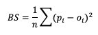
Here, pi is the forecast probability while oi is the binary representation of the observance of the event (1 if the event occurred, 0 if the event did not occur). This summation score is negatively oriented, with a 0 indicating perfect accuracy and 1 showing complete inaccuracy. The score is sensitive to the frequency of an event and should only be used on forecast-observation datasets that boast a substantial number of event samples.

Through substitutions, BS can be decomposed into three terms that describe the reliability, resolution, and uncertainty of the forecasts (more on these attributes can be found in the Attributes of Forecast Quality section). This decomposition is given as

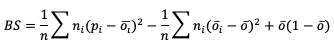
where the three terms are reliability, resolution, and uncertainty, respectively. ni is the count of probabilistic forecasts that fall into each probabilistic bin. See how to use this statistic in METplus!

Ranked Probability Score

A second statistical score to use for probabilistic forecasts is the Ranked Probability Score (RPS). This score differs from BS in that it allows the verification of multicategorical probabilistic forecasts where BS strictly pertains to binary probabilistic forecasts. While the RPS formula  is based on a squared error at its core (similar to BS), it remains sensitive to the distance between the forecast probability and the observed event space (1 if the event occurred, 0 if it did not) by calculating the squared errors in cumulative probabilistic forecast and observation space. This formulation is represented in the following equation

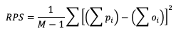
Note how RPS reduces to BS when there are only two forecast categories evaluated. In the equation, M denotes the number of categories the forecast is divided into. Because of the squared error usage, RPS is negative orientated with a 0 indicating perfect accuracy and 1 showing complete inaccuracy. See how to use this statistic in METplus!

Continuous Ranked Probability Score

Similar to the RPS’s approach to provide a probabilistic evaluation of multicategorical forecasts and the BS formulation as a statistic for binary probabilistic forecasts, the Continuous Ranked Probability Score (CRPS) provides a statistical measure for forecasts in the continuous probabilistic space. Theoretically this is equivalent to evaluating multicategorical forecasts that extend across an infinite number of categories that are infinitesimally small. When it comes to application, however, it becomes difficult to express mathematically a closed form of CRPS. Due to this restriction, CRPS often utilizes an assumption of a Gaussian (i.e. normal) distribution in the dataset and is presented as

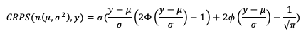
In this equation we use μ and σ to denote the mean and standard deviation of the forecasts, respectively, ɸ to represent the cumulative distribution function (CDF ) and 𝚽 to represent the probability density function (PDF) of the normal distribution. If you’ve previously evaluated meteorological forecasts, you know that the assumption that the dataset can be described by a Gaussian distribution is not always correct. Temperature and pressure variable fields, among others, can usually take advantage of this CRPS definition as they often are well fitted by a Gaussian distribution. But other important meteorological fields, such as precipitation, do not. Using statistics that are created with an incorrect assumption will produce, at best, misleading results. Be sure that your dataset follows a Gaussian distribution before relying on the above definition of CRPS!

The CRPS is negatively oriented with a 0 indicating perfect accuracy and 1 showing complete inaccuracy. See how to use this statistic in METplus!

Probabilistic Skill Scores

Some of the previously mentioned verification statistics for probabilistic forecasts can be used to compute skill scores that are regularly used. All of these skill scores use the same general equation format of comparing their respective score results to a base or reference forecast, which can be climatology, a “random” forecast, or any other comparison that could provide useful information.

Brier Skill Score

The Brier Skill Score (BSS) measures the relative skill of the forecast compared to a reference forecast. It’s equation is simple and follows the general skill score format:

Compared to the BS equation, the range of values for BSS differs: the range is from negative infinity to 1, with 1 showing a perfect skill and 0 showing no discernable skill compared to a reference forecast. See how to use this skill score in METplus!

Ranked Probability Skill Score

Similar to the BSS, the Ranked Probability Skill Score (RPSS) follows the general skill score equation formulation, allowing a comparison between a chosen reference forecast and the forecast of interest:

RPSS measures the improvement/degradation of the ranked probability forecasts compared to the skill of a reference forecast. As with BSS, RPSS ranges from negative infinity to 1, with a perfect score of 1, and a score of zero indicating no improvement of forecast performance relative to the reference forecast. See how to use this skill score in METplus!

METplus Solutions for Probabilistic Forecast Verification

If you utilize METplus verification capabilities to evaluate probabilistic forecasts, you may find that your final statistical values are not exactly the same as when you compute the same statistic by pencil and paper or in a separate statistical program. These very slight differences are due to how METplus handles probabilistic information. 

MET is coded to utilize categorical forecasts, creating contingency tables and using the counts in each of the contingency table cells (hits, misses, false alarms, and correct rejections) to calculate the desired verification statistics. This use extends to probabilistic forecasts as well and aids in the decomposition of statistics such as Brier Score (BS) into reliability, resolution, and uncertainty (more information on that decomposition can be found here). 

MET requires users to provide three conditions for probabilistic forecasts. The first of these conditions is an observation variable that is either a 0 or 1 and a forecast variable that is defined on a scale from 0 to 1. In MET, this boolean is prob and METplus Wrappers utilizes the variable FCST_IS_PROB. In MET prob can also be defined as a dictionary with more information on how to process the probabilistic field; please review this section of the User’s Guide for information. 

The second condition is the thresholds to evaluate the probabilistic forecasts across. Essentially this is where METplus turns the forecast probabilities into a binned, categorical evaluation. At its most basic usage in a MET configuration file, this looks like

cat_thresh = ==0.1; 

which would create 10 bins of equal width. Users have multiple options for setting this threshold and should review this section of the User’s Guide for more information. It’s important to note that when it comes to evaluating a statistic like BS, METplus does not actually use the forecasts’ probability value; instead, it will use the midpoint of the bin width between the thresholds for the probabilistic forecasts. To understand what this looks like in METplus, let's use the previous example where 10 bins of equal width were created. When calculating BS, METplus will evaluate the first probability bin as 0.05, the midway point between the first bin (0.0 to 0.1). The next probability value would be 0.15 (the midway point between 0.1 and 0.2), and so on. MET utilizes an equation of BS that is described in more detail in the MET Appendix which evaluates to the same result as the BS equation provided in the Verification Statistics for Probabilistic Forecasts section of this guide {provide link to previous section here} if the midpoints of the bins are used as the probability forecast values. All of this is to stress that a proper selection of bin width (and the accompanying mid-point of those bins) will ultimately determine how meaningful your resulting BS value is; after all, what would the result be if the midpoint of a bin was 0.1 and many of the forecasts values were 0.1? What contingency table bin will they count towards?

The final condition users need to provide to MET for probabilistic forecasts is a threshold for the observations. As alluded to in the second condition, users can create any number of thresholds to evaluate the probabilistic forecasts. Combined with the observation threshold which determines an event observation from non-event observation, an Nx2 contingency table will be created, where N is the number of probabilistic bins for the forecasts and 2 is the event, non-event threshold set on the observations.

Now that you know a bit more about probabilistic forecasts and the related statistics as well as how MET will process them, it’s time to show how you can access those same statistics in METplus!

In order to better understand the delineation between METplus, MET, and METplus wrappers which are used frequently throughout this tutorial but are NOT interchangeable, the following definitions are provided for clarity:

• METplus is best visualized as an overarching framework with individual components. It encapsulates all of the repositories: MET, METplus wrappers, METdataio, METcalcpy, and METplotpy.
• MET serves as the core statistical component that ingests the provided fields and commands to compute user-requested statistics and diagnostics.
• METplus wrappers is a suite of Python wrappers that provide low-level automation of MET tools and plotting capability. While there are examples of calling METplus wrappers without any underlying MET usage, these are the exception rather than the rule.

MET solutions

The MET User’s Guide provides an Appendix that dives into statistical measures that it calculates, as well as the line type it is a part of. Statistics are grouped together by application and type and are available to METplus users in line types. For the probabilistic-related statistics discussed in this section of the tutorial, MET provides the Contingency Table Counts for Probabilistic forecasts (PCT) line type, and the Contingency Table Statistics for Probabilistic forecasts (PSTD) line types. The PCT line type is critical for checking if the thresholds for the probabilistic forecasts and observations produced contingency table counts that reflect what the user is looking for in probabilistic verification. Remember that these counts are ultimately what determine the statistical values found in the PSTD line type.

As for the statistics that were discussed in the Verification Statistics section, the following are links to the User’s Guide Appendix entry that discusses their use in MET. Note that Continuous Ranked Probability Score (CRPS) and Continuous Ranked Probability Skill Score (CRPSS) appear in the Ensemble Continuous Statistics (ECNT) line type and can only be calculated from the Ensemble-Stat tool, while Ranked Probability Score (RPS) and Ranked Probability Skill Score (RPSS) appear in their own Ranked Probability Score (RPS) line type output that is also only accessible from Ensemble-Stat. RPSS is not discussed in the MET USer’s Guide Appendix and is not linked below, while discussion of CRPSS is provided to users in the existing documentation in the MET User’s Guide Appendix:

• BS
• RPS
• CRPS
• BSS
• CRPSS

METplus Wrapper Solutions

The same statistics that are available in MET are also available with the METplus wrappers. To better understand how MET configuration options for statistics translate to METplus wrapper configuration options, you can utilize the Statistics and Diagnostics Section of the METplus wrappers User’s Guide, which lists all of the available statistics through the wrappers, including what tools can output what statistics. To access the line type through the tool, find your desired tool in the list of available commands for that tool. Once you do, you’ll see the tool will have several options that contain _OUTPUT_FLAG_. These will exhibit the same behavior and accept the same settings as the line types in MET’s output_flag dictionary, so be sure to review the available settings to get the line type output you want.

METplus Examples of Probabilistic Forecast Verification

The following two examples show a generalized method for calculating probabilistic statistics: one for a MET-only usage, and the same example but utilizing METplus wrappers. These examples are not meant to be completely reproducible by a user: no input data is provided, commands to run the various tools are not given, etc. Instead, they serve as a general guide of one possible setup among many that produce probabilistic statistics.

If you are interested in reproducible, step-by-step examples of running the various tools of METplus, you are strongly encouraged to review the METplus online tutorial that follows this statistical tutorial, where data is made available to reproduce the guided examples.

In order to better understand the delineation between METplus, MET, and METplus wrappers which are used frequently throughout this tutorial but are NOT interchangeable, the following definitions are provided for clarity:

• METplus is best visualized as an overarching framework with individual components. It encapsulates all of the repositories: MET, METplus wrappers, METdataio, METcalcpy, and METplotpy.
• MET serves as the core statistical component that ingests the provided fields and commands to compute user-requested statistics and diagnostics.
• METplus wrappers is a suite of Python wrappers that provide low-level automation of MET tools and plotting capability. While there are examples of calling METplus wrappers without any underlying MET usage, these are the exception rather than the rule.

MET Example of Probabilistic Forecast Verification

Here is an example that demonstrates probabilistic forecast verification using MET.

For this example, we will use two tools: Gen-Ens-Prod, which will be used to create uncalibrated probability forecasts, and Grid-Stat, which will verify the forecast probabilities against an observational dataset. The “uncalibrated” term means that the probabilities gathered from Gen-Ens-Prod may be biased and will not perfectly reflect the true probabilities of the forecasted event. To avoid complications with assuming gaussian distributions on non-gaussian variable fields (i.e. precipitation), we’ll verify the probability of a CONUS 2 meter temperature field from a global ensemble with 5 members with a threshold of greater than 10 degrees Celsius.

Starting with the general Gen-Ens-Prod configuration file, the following would resemble the minimum necessary settings/changes for the ens dictionary:

We can see right away that Gen-Ens-Prod is different from most MET tools; it utilizes only one dictionary to process fields (as opposed to the typical forecast and observation fields). This is by design and follows the guidance that Gen-Ens-Prod generates ensemble products, rather than verifying ensemble forecasts (which is left for Ensemble-Stat). Even with this slight change, the name and level entries are still set the same as they would be in any MET tool; that is, according to the information in the input files (e.g., a variable field named TMP on the second vertical level). The cat_thresh entry reflects an interest in 2 meter temperatures greater than 10 degrees Celsius. We’ve also included a convert function which will convert the field from its normal output of Kelvin to degrees Celsius. If you’re interested in learning more about this tool, including in-depth explanations of the various settings, please review the MET User’s Guide entry for Gen-Ens-Prod or get a hands-on experience with the tool in the METplus online tutorial.

Let’s also utilize the regrid dictionary, since we are only interested in CONUS and the model output is global:

More discussion on how to properly use the regrid dictionary and all of its associated settings can be found in the MET User’s Guide.

All that’s left before running the tool is to set up the ensemble_flag dictionary correctly:

In the first half of this example, we have told MET to create a CONUS 2 meter temperature field count from 0.0 to 1.0 at each grid point representing how many of the ensemble members forecast a temperature greater than 10 degrees Celsius. So with this configuration file we’ll create a probability field based on ensemble member agreement and disagreement.

The output from Gen-Ens-Prod is a netCDF file whose content would contain a variable field as described above. It should look something like the following:

With this new MET field output, we can verify this uncalibrated probabilistic forecast for 2 meter temperatures greater than 10 degrees Celsius against an observation dataset in Grid-Stat.

Now for the actual verification and statistical generation we turn to Grid-Stat. Starting with the general Grid-Stat configuration file, let’s review how we might set the fcst dictionary:

In this example we see the name of the variable field from the Gen-Ens-Prod tool’s netCDF output file, TMP_Z2_ENS_FREQ_gt10, set as the forecast field name. The prob setting informs MET to process the field as probabilistic data, which requires an appropriate categorical threshold creation. Using “==0.1” means MET will create 10 bins from 0 to 1, each with a width of 0.1. Recall from previous discussion on how MET evaluates probabilities that MET will use the midpoints of each of these bins to evaluate the forecast. Since the forecast data probabilistic resolution is 0.1, the use of 0.05 as the evaluation increment is reasonable. 

Now let’s look at a possible setup for the obs dictionary:

Notice that we’ve used the convert function again to change the original Kelvin field to degrees Celsius, along with the appropriate variable field name and second vertical level request. For the threshold we re-use the same value that was originally used to create the forecast probabilities, greater than 10 degrees Celsius. This matching value is important as any other comparison would mean an evaluation between two inconsistent fields.

Since the forecast and observation fields are on different grids, we’ll utilize the regrid dictionary once again to place everything on the same evaluation gridspace:

Finally, we choose the appropriate flags in the output_flag dictionary to gain the probabilistic statistics:

With a successful run of MET, we should find a .stat file with two rows of data; one for the PCT line type that will provide information on the specific counts of observations that fell into each of the forecast’s probability bins, and one for the PSTD line type which has some of the probabilistic measures we discussed in this chapter. The content might look similar to the following:

Note that the rows have been truncated and would normally hold more information to the left of the FCST_THRESH entry. But from this snippet we see that there were 103,936 matched pairs for the comparison, with PCT line type showing many of the observations falling in the “no” category of the 0 to 0.1 bin and the “yes” category of the 0.9 to 1.0 bin. In fact, less than seven percent of the matched pairs fell into categories outside of these two. This distribution tells us that the model was very confident in its probabilities, supported by the observations. This is reflected in the outstanding statistical values of the PSTD line type, including a 0.0019261 Reliability value (recall that a zero is ideal and indicates less differences between the average forecast probability and the observed average frequency) and a near-perfect Brier score of 0.019338 (0 being a perfect score). There is some room for improvement, as reflected in a 0.231 Resolution value (remember that this is the measure of the forecast’s ability to resolve different observational distributions given a change in the forecast value, and a larger value is desirable). For a complete list of all of the statistics given in these two line types, review the MET User’s Guide entries for the PCT and PSTD line types.

METplus Wrapper Example of Probabilistic Forecast Verification

To achieve the same success as the previous example, but utilizing METplus wrappers instead of MET, very few adjustments would need to be made. In fact, approaching this example utilizing the wrappers simplifies the problem, as one configuration file can be used to generate the desired output from both tools.

Starting with variable fields, we would need to set the _VAR1 settings appropriately. Since we are calling two separate tools, it would be best practice to utilize the individual tool’s variable field settings, as seen below:

You can see how the GenEnsProd field variables start with the prefix ENS_, and the GridStat wrapper field variables have _GRID_STAT_ in their name. Those GridStat field settings are also clearly separated into forecast (FCST_) and observation (OBS_) options. Note how from the MET-only approach we have simply changed what the setting name is, but the same values are utilized, all in one configuration file.

To recreate the regridding aspect of the MET example, we would call the wrapper-appropriate regridding options:

Because the loop/timing information is controlled inside the configuration file for METplus wrappers (as opposed to MET’s non-looping option), that information must also be set accordingly. This is also an appropriate time to set up the calls to the wrappers in the desired order:

Now a one time loop will be executed with a forecast lead time of 24 hours, matching the forecast and observation datasets’ relationship.

One part that needs to be done carefully is the input directory and file name template for GridStat. This is because we are relying on the output from the previous wrapper, GenEnsProd, and need to set the variable accordingly. As long as the relative value is used, this process becomes much simpler, as shown:

These commands will tie the input for GridStat to wherever the output from GenEnsProd was set.

Finally we set up the correct output requests for each of the tools:

And with a successful run of METplus we would arrive at the same output as we obtained from the MET-only example. This example once again highlights the usefulness of METplus wrappers in chaining multiple tools together in one configuration file.