Verification Statistics for Multicategorical Forecasts

In order to make sense of how the statistics are modified when evaluating multiple categories, it will help to look at how the contingency table changes. The generalized contingency table for a three category table will look like the following:

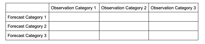
A similar table could be constructed for comparisons of four, five, six, and so on, categories. Some statistical calculations are more easily computed when forecasts and observations are restricted to two options (as was the case in binary categorical forecasts), so one less common approach for a multi-category contingency table is to process the full table  into multiple instances of 2x2 grids,  focusing on one forecast category at a time. This way, each forecasted event or category can have scalar attributes calculated, as well as skill scores that reflect the entire forecast’s quality across the multiple categories. This is not a valid approach for calculating, among others, Heidke Skill Score and Gilbert Skill Score, but is considered here for a well-rounded approach to multicategorical verification.

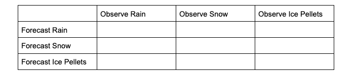
To demonstrate how scalar attributes are calculated for a multicategory forecast, imagine a scenario where the forecast can call for three separate precipitation types: rain, snow, and ice pellets. For this scenario, forecasts and observations of no precipitation are ignored (i.e., this evaluation is conditioned on some type of precipitation both occurring and being forecasted).

The contingency table would look like the following:

To extract the scalar attributes for rain, the simplified, 2x2 contingency table would look like this:

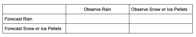
The same simplification can be done for snow and ice pellets. As this new 2x2 contingency table demonstrates, by reducing the multicategorical options to the binary choices of each forecasted event (e.g., did the forecast predict rain rather than snow or ice pellets, did the forecast predict snow rather than rain or ice pellets, did the forecast predict ice pellets rather than rain or snow) and evaluating the corresponding observations, scalar statistics such as POD, Bias, etc. can be calculated in the same method as the binary categorical forecasts. 

One of the unique scalar statistics that does not need a contingency table simplification is Accuracy (Acc). This is due to its definition, which, when presented in its general format, becomes:

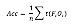
Note that t(FiOi) is the number of forecasts in category i of the multicategory contingency table that had an observation of Oi and n is the total number of occurrences and non-occurrences.

With this general format of Accuracy, essentially we seek to answer the question “how capable was the forecast at selecting the exact category?” To demonstrate how this would look in a 3x3 contingency table, let’s return to the previous scenario of a three precipitation type forecast. A perfect Accuracy forecast would have nonzero values only in the “Forecast Rain, Observation Rain”, “Forecast Snow, Observation Snow”, and “Forecast Ice Pellets, Observation Ice Pellets”  cells, with the remaining cells being zero. The same top-left corner to lower-right corner of nonzero cells pattern would exist in the simplified 2x2 contingency table. Because no information about the forecast’s Accuracy is lost for the full count of forecast categories, Accuracy is the only scalar statistic that METplus will calculate from the full multicategory contingency table. See how to use this statistic in METplus! 

Multicategorical Skill Scores

While some statistics for multicategorical forecasts require simplifying the contingency table to two-categories, and therefore only show the forecast’s quality in respect to the individual category, certain skill scores are designed to evaluate forecasts with multiple categories, allowing the skill score to reflect the quality of the entire forecast spectrum.

Heidke Skill Score (HSS)

HSS has a general form to accommodate multicategory forecasts. While more computationally intense than the two-category equation provided, the multi-category formulation is also based on comparison of the percent correct in the forecast relative to the proportion correct that would be achieved by a “random” forecast. The relative comparison is often with sources other than a “random” forecast, including older versions of a model and climatology. This general form is

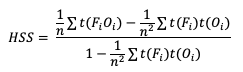
Note that t(FiOi) is the number of forecasts in category i of the multicategory contingency table that had an observation of Oi, t(Fi) is the total number of forecasts in category i, and n is the total number of occurrences and non-occurrences.

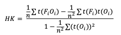
Hanssen-Kuipers Discriminant (HK)

Similarly, HK is generalized to

Gerrity Skill Score

The Gerrity Skill Score is designed specifically for multicategory forecasts. While it is not as easily calculated as HSS and HK, it is useful for demonstrating the ability of the forecasts to delineate the correct event category when compared to random chance. The Gerrity Skill Score properly penalizes a forecast that has more than two options for an event, something not captured in the generalized forms of HSS or HK. This is achieved through the use of weights, sj,j, which correspond to correct forecasts, and sj,i, which represent weights for incorrect forecasts. These weights are given as

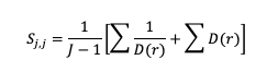
and

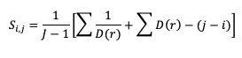
where D(r) is the likelihood ratio using dummy summation index r, calculated using

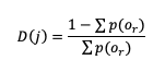
where p(or) is the probability of a sample climatology.

Finally, the Gerrity Skill Score is computed through summing the product of the scoring weights and their corresponding joint probability distribution. That distribution is found by taking each count of the contingency table cell and dividing it by the total number of occurrences and non-occurrences across all cells, n. See how to use these statistics in METplus!

METplus solutions for Multicategorical Forecast Verification

One important note regarding how to define multicategorical thresholds within the MET and METplus wrapper configuration files should be discussed. METplus requires that when multiple thresholds are listed using the cat_thresh variable to calculate any multicategorical line types, the thresholds must be monotonically increasing and use the same inequality type. This is done in order to ensure that the thresholds create unique and discrete bins of values, rather than overlapping thresholds that do not provide any sound statistical value. In practice, this means that the following two examples would result in a METplus error:

Example 1.

Example 2.

In example 1, the thresholds decrease with each entry which violates the requirement of monotonically increasing. With a simple reordering of the thresholds, example 1 can use the same thresholds and run with success:

In example 2, the final threshold uses a different inequality than the other two thresholds which violates the requirement that all multicategorical thresholds use the same inequality type. This rewrite of example 2 will provide the same information desired from the original thresholds, but will now successfully run in METplus:

This time, the rewrite changed the final inequality to match the first two while also keeping the final bin of values that METplus will calculate, >=15.5, consistent with the desired information. More information on how MET creates the value bins from multicategory thresholds is provided in the MET example of Multicategorical Forecast Verification.

Now that you know a bit more about verification measures for multicategorical, deterministic forecasts, it’s time to show how you can access those same statistics in METplus!

In order to better understand the delineation between METplus, MET, and METplus wrappers which are used frequently throughout this tutorial but are NOT interchangeable, the following definitions are provided for clarity:

• METplus is best visualized as an overarching framework with individual components. It encapsulates all of the repositories: MET, METplus wrappers, METdataio, METcalcpy, and METplotpy.
• MET serves as the core statistical component that ingests the provided fields and commands to compute user-requested statistics and diagnostics.
• METplus wrappers is a suite of Python wrappers that provide low-level automation of MET tools and plotting capability. While there are examples of calling METplus wrappers without any underlying MET usage, these are the exception rather than the rule

MET solutions

The MET User’s Guide provides an Appendix that dives into statistical measures that it calculates, as well as the line type it is a part of. Statistics are grouped together by application and type and are available to METplus users in line types. To delineate between the calculation method for binary categorical and multicategorical forecast skill scores, METplus has two pairs of separate, but similar line types. As discussed in detail in the Binary Categorical forecasts section, the Contingency Table Statistics (CTS) line type and Contingency Table Counts (CTC) line type are for users who want single category forecast statistics. It’s important to note that the CTS line type must also be utilized by users who want scalar statistics from multicategorical forecasts, except for Accuracy. To accomplish this, simply follow the guidance listed in the Verification Statistics section for Multicategorical Forecasts. The complements to CTS and CTC in the multicategory group are the aptly named Multicategory Contingency Table Statistics (MCTS) line type and Multicategory Contingency Table Counts (MCTC) line type. Similar to the CTC, MCTC allows direct access to each of the counts from the contingency table of multicategorical forecasts. MCTS contains all of the skill scores that were discussed in the Multicategorical Verification statistics section, as well as the scalar statistic Accuracy, which are linked to their appendix description here for your convenience (except for Gerrity, which does not appear in the appendix):

• Acc
• HK
• HSS
• Gerrity

METplus Wrapper Solutions

The same statistics that are available in MET are also available with the METplus wrappers. To better understand how MET configuration options for statistics translate to METplus wrapper configuration options, you can utilize the Statistics and Diagnostics Section of the METplus wrappers User’s Guide, which lists all of the statistics available through the wrappers, including which tools can output which statistics. To access the line type through the tool, find your desired tool in the list of available commands for that tool. Once you do, you’ll see the tool will have several options that contain _OUTPUT_FLAG_, which will exhibit the same behavior and accept the same settings as the line types in MET’s output_flag dictionary, so be sure to review the available settings to get the line type output you want.

The following two examples show a generalized method for calculating multicategorical statistics: one for a MET-only usage, and the same example but utilizing METplus wrappers. These examples are not meant to be completely reproducible by a user: no input data is provided, commands to run the various tools are not given, etc. Instead, they serve as a general guide of one possible setup among many that produce multicategorical statistics.

If you are interested in reproducible, step-by-step examples of running the various tools of METplus, you are strongly encouraged to review the METplus online tutorial that follows this statistical tutorial, where data is made available to reproduce the guided examples.

In order to better understand the delineation between METplus, MET, and METplus wrappers which are used frequently throughout this tutorial but are NOT interchangeable, the following definitions are provided for clarity:

• METplus is best visualized as an overarching framework with individual components. It encapsulates all of the repositories: MET, METplus wrappers, METdataio, METcalcpy, and METplotpy.
• MET serves as the core statistical component that ingests the provided fields and commands to compute user-requested statistics and diagnostics.
• METplus wrappers is a suite of Python wrappers that provide low-level automation of MET tools and plotting capability. While there are examples of calling METplus wrappers without any underlying MET usage, these are the exception rather than the rule.

MET Example of Multicategorical Forecast Verification

Here is an example that demonstrates multicategorical forecast verification in MET.

For this example, let’s use Point-Stat. Assume we wanted to verify a multicategory forecast of wind speeds over the ocean. Specifically of interest are speed thresholds of near gale force (13.9 m/s), gale force (17.2 m/s), tropical storm (24.5 m/s), and hurricane (32.7 m/s). Starting with the general Point-Stat configuration file, the following would resemble minimum necessary settings/changes for the fcst and obs dictionaries:

In this example, the forecast field name in the forecast input file is named WIND, and is set accordingly in the fcst dictionary. Wind speed is one of the unique variables in METplus that can be calculated from the u and v components of a grib1 or grib2 file if wind speed is not present in the file. Assuming the input file is in a grib1 or grib2 format, MET will first check if a variable field WIND is present; if it is, MET will use the values in that field for analysis. If not, MET will check for the u-component (UGRD) and v-component (VGRD) fields and if found, compute the wind speed field for analysis. A level of Z10 is used to grab the vertical level of 10 that WIND appears on, which for this input file corresponds to the 10 meter level. Finally, cat_thresh, which controls the categorical threshold used to create the multicategory contingency table, is set to four separate thresholds, with each value corresponding to one of the wind speed thresholds of interest. The example’s chosen thresholds assume that the wind speed units in the file are in meters per second. All of the additional fcst field entries from the general Point-Stat configuration file were removed. Note how MET uses four thresholds to creates five unique, discrete bins of wind speeds with a contingency table that would look like the following:

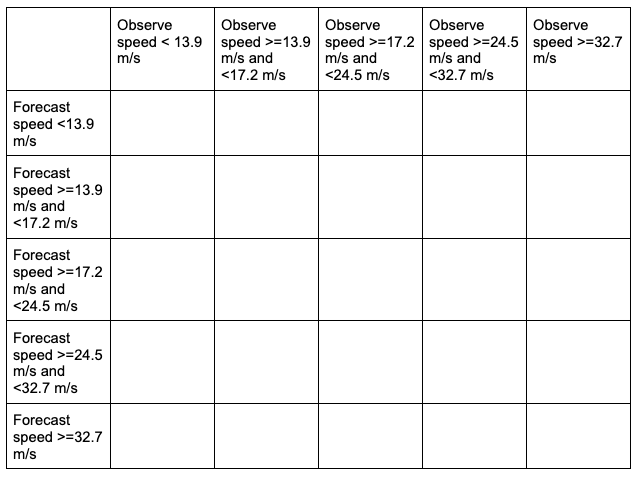
The table includes a “hidden” bin containing wind speeds less than 13.9 m/s that is not explicitly listed by a threshold in the MET settings, but rather implied: each of these bins is mutually exclusive and together they entail the complete real number line. This is why it is important to remember the “monotonically increasing and same inequality type” requirement when setting multicategorical forecast thresholds in METplus. For more discussion on this, review the METplus Solutions for Multicategorical Forecast Verification section.

The obs dictionary is simply copying the settings from the fcst dictionary, which is a method that can be used if both the forecast and observation input files share the same variable structure and file type (e.g. both inputs use the WIND variable name, in m/s, with the Z10 level corresponding to the 10 meter level).

Now all that’s necessary is to adjust the output_flag dictionary settings to have Point-Stat print out the desired line types:

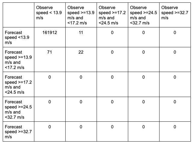
In this example, we have told MET to output the MCTC and MCTS line types, which will produce one .stat file with the two line types that were selected. The MCTC line would look something like:

While the stat file full header column contents are discussed in the User’s Guide, the MCTC line types are the final columns of the line beginning after the “MCTC” column. The first value is MET’s TOTAL column which is the “total number of matched pairs”. You might better recognize this value as n, the summation of every cell in the contingency table. The following value is the number of dimensions or bins of the contingency table. As discussed above, providing four categorical thresholds creates a 5x5 contingency table. That means that we expect, and receive, 25 cells of data that make up the contingency table. They are listed starting with the lowest forecast and observation threshold pair, with increasing observation thresholds starting first. For the contingency table provided in this example, it would look like the following:

Note that the final column of the MCTC line type, EC_VALUE, is only relevant to users verifying probabilistic data with the HSS_EC skill score.

The MCTS line type is also present in the .stat file as the second row. In this example, the contents would be:

Compared to the statistics available in the CTC line type for dichotomous categorical forecasts, fewer verification statistics can be applied to a multicategorical contingency table, since most of the  contingency table verification statistics require a simplified 2x2 contingency table. The columns that are available in the MCTS line type are listed in the MET User’s Guide guidance for the MCTS line type. After the declaration of the line type (MCTS), the familiar TOTAL or n column, and the number of bins created from the thresholds provided, we find Accuracy, HK, HSS, the Gerrity Skill Score, and HSS_EC, all with their appropriate lower and upper confidence intervals and the bootstrap confidence intervals. Accuracy has an additional two columns that give the normal confidence limits in addition to the bootstrap confidence limits. Note that because the bootstrap library’s n_rep variable was kept at its default value of 0, bootstrap methods were not used and appear as NA in the stat file. While all of these statistics could be obtained from the MCTC line type values with additional post-processing, the simplicity of having all of them already calculated and ready for additional group statistics or to advise forecast adjustments is one of the many advantages of using the METplus system.

METplus Wrapper Example of Multicategorical Forecast Verification

To achieve the same success as the previous example but utilizing METplus wrappers instead of MET, very few adjustments would need to be made. Starting with the standard PointStat configuration file, we would need to set the _VAR1 settings appropriately:

Note how the BOTH option is utilized here (as opposed to individual FCST_ and OBS_ settings) since the forecast and observation datasets utilize the same name and level information. Because the loop/timing information is controlled inside the configuration file for METplus wrappers (as opposed to MET’s non-looping option), that information must also be set accordingly:

Finally, the desired line types need to be selected for output. In the wrappers, that looks like this:

With a proper setting of the input and output directories, file templates, and a successful run of METplus, the same .stat output file that was created in the MET example would be produced here, complete with MCTC and MCTS line type rows.