UFS Short-Range Weather (SRW) Practical Session Guide
UFS Short-Range Weather (SRW) Practical Session GuideWelcome to the Unified Forecast System (UFS) Short-Range Weather (SRW) Application Practical Session Guide
September 20-24, 2021
Session 1: Set up and run a 2 day simulation with significant severe weather across the Contiguous United States (CONUS) from 15-16 June 2019. This forecast uses a predefined Rapid Refresh Forecast System (RRFS) CONUS grid with 25 km resolution, the FV3_GFS_v15p2 Common Community Physics Package (CCPP) physics suite, and FV3GFS initial and lateral boundary conditions.
Session 2: Describes how to change the predefined grid resolution, and then progresses to changing the physics suite and the external models for generating initial conditions (ICs) and lateral boundary conditions (LBCs). Users will learn how to define a custom regional Extended Schmidt Gnomonic (ESG) grid.
Session 3: Explores how to customize the Unified Post Processor (UPP) output by adding/removing fields/levels. Describes how to change a physics scheme in an existing Suite Definition File (SDF).
Throughout this training, please note, blocks of text follow these conventions:
-
Black background with white text is the command you should run.
-
Gray background with black text is the output you should see when you run the command.
-
Yellow background contains important/helpful tips.
-
Blue background with black text is additional information.
You will use the NCAR HPC computer, Cheyenne, to download, compile, and run the SRW App. Click on "Session 1" to get started.
Session 1
Session 1Setup and Run the Workflow
This session will enable you to run a two-day simulation with significant severe weather across the Contiguous United States (CONUS) from 15-16 June 2019. This test case uses FV3GFS initial and lateral boundary conditions in GRIB2 format. The simulation is configured for the predefined RRFS CONUS grid with 25 km resolution, and the FV3_GFS_v15p2 CCPP physics suite. The code base includes the UFS Weather Model, with pre- and post-processing, running with the regional workflow. In order to perform the test case, you will run the Short-Range Weather Application for 48 hours.
0. Log In To Cheyenne
0. Log In To CheyenneFrom a terminal:
And follow the instructions you received (Yubikey, Duo, other) to authenticate and complete the login.
* Welcome to Cheyenne - June 15,2021
******************************************************************************
Today in the Daily Bulletin (dailyb.cisl.ucar.edu)
- Opportunity for university researchers on NCAR’s Derecho supercomputer
- Where to run small jobs that only use CPUs
HPSS Update: 108 days until HPSS will be decommissioned.
Quick Start: www2.cisl.ucar.edu/resources/cheyenne/quick-start-cheyenne
User environment: www2.cisl.ucar.edu/resources/cheyenne/user-environment
Key module commands: module list, module avail, module spider, module help
CISL Help: support.ucar.edu -- 303-497-2400
--------------------------------------------------------------------------------
my_var="hello"
while in csh/tcsh, we use
set my_var="hello"
For convenience, set some environment variables to more easily navigate in your work space on Cheyenne. In this tutorial, we will use /glade/scratch:
SR_WX_APP_TOP_DIR=$SCRATCH_DIR/ufs-srweather-app
where $USER is your login/username, and $SR_WX_APP_TOP_DIR is the path in which you will clone the GitHub repository in the next step. Go to your work space on Cheyenne:
1. Clone the Code
1. Clone the CodeEstimated time: 5 minutes
The necessary source code is publicly available on GitHub. To clone the ufs-v1.0.1 branch of the ufs-srweather-app repository:
cd ufs-srweather-app
For convenience, set:
The UFS SRW App uses components from multiple repositories, including: the regional workflow, the UFS_UTILS pre-processor utilities, the UFS Weather Model, and the Unified Post Processor (UPP). Obtaining the necessary external repositories is simplified by the use of manage_externals:
The checkout_externals script uses the configuration file Externals.cfg in the top level directory and will clone the regional workflow, pre-processing utilities, UFS Weather Model, and UPP source code into the appropriate directories under your regional_workflow and src directories. The process will take several minutes and show the following progress information on the screen:
Checking status of externals: regional_workflow, ufs-weather-model, ufs_utils, emc_post,
Checking out externals: regional_workflow, ufs-weather-model, ufs_utils, emc_post,
Once the externals have been downloaded, you can proceed to the next step, building the executables.
2. Build the Executables
2. Build the ExecutablesEstimated time: 20-25 minutes
Instructions for loading the proper modules and/or setting the correct environment variables can be found in the env/ directory in files named build_<platform>_<compiler>.env. The commands in these files can be directly copy-pasted to the command line or the file can be sourced.
cp build_cheyenne_intel.env build_cheyenne_intel_tcsh.env
Make the following changes to build_cheyenne_intel_tcsh.env. Change
export CMAKE_CXX_COMPILER=mpicxx
export CMAKE_Fortran_COMPILER=mpif90
export CMAKE_Platform=cheyenne.intel
to
setenv CMAKE_CXX_COMPILERmpicxx
setenv CMAKE_Fortran_COMPILER mpif90
setenv CMAKE_Platform cheyenne.intel
The modified script can then be sourced as follows:
source ./env/build_cheyenne_intel_tcsh.env
to set the build environment.
Build the executables as follows (for both bash and csh/tcsh users):
cd build
Run cmake to set up the Makefile, then run make:
make -j 4 >& build.out &
Output from the build will be in the $SR_WX_APP_TOP_DIR/build/build.out file. When the build completes, you should see the forecast model executable NEMS.exe and eleven pre- and post-processing executables in the $SR_WX_APP_TOP_DIR/bin directory.
3. Generate the Workflow Experiment
3. Generate the Workflow ExperimentEstimated time: 15 minutes
Generating the workflow requires three steps:
- Set experiment parameters in config.sh
- Set Python and other environment parameters
- Run the generate_FV3LAM_wflow.sh script
The workflow requires a file called config.sh to specify the values of your experiment parameters. Make a copy of the example template config.community.sh file provided in the $SR_WX_APP_TOP_DIR/regional_workflow/ush directory (from the build directory):
cp config.community.sh config.sh
Edit the config.sh file on Cheyenne for running the FV3_GFS_v15p2 physics suite for 48 hours starting at 00 UTC on 15 June 2019 on a 25 km predefined CONUS domain. Since this is the default case, only the following variables need to be modified in config.sh:
ACCOUNT="NJNT0008"
USE_USER_STAGED_EXTRN_FILES="TRUE"
EXTRN_MDL_SOURCE_BASEDIR_ICS="/glade/p/ral/jntp/UFS_SRW_app/staged_extrn_mdl_files/FV3GFS"
EXTRN_MDL_SOURCE_BASEDIR_LBCS="/glade/p/ral/jntp/UFS_SRW_app/staged_extrn_mdl_files/FV3GFS"
where ACCOUNT is an account you can charge. We will be using pre-staged initialization data, so uncomment USE_USER_STAGED_EXTRN_FILES="TRUE".
EXTRN_MDL_SOURCE_BASEDIR_ICS and EXTRN_MDL_SOURCE_BASEDIR_LBCS contain the locations of the initial and lateral boundary conditions, and EXTRN_MDL_FILES_ICS and EXTRN_MDL_FILES_LBCS contain the filenames of the initial and lateral boundary conditions.
Load the appropriate Python environment for Cheyenne:
If you see something like:
Do you wish to add it to the registry (y/N)?
This will occur if this is the first time you have used the NCAR Python Library (NPL), type y, to get the following output:
Now using NPL virtual environment at path:
/glade/p/ral/jntp/UFS_SRW_app/ncar_pylib/regional_workflow
Use deactivate to remove NPL from environment
The workflow can be generated with the command:
The generated workflow will be located in ${SR_WX_APP_TOP_DIR}/../expt_dirs/${EXPT_SUBDIR} where ${SR_WX_APP_TOP_DIR} is the directory where the ufs-srweather-app was cloned in Step 1, and ${EXPT_SUBDIR} is the experiment name set above in the config.sh file: test_CONUS_25km_GFSv15p2
4. Run the Workflow
4. Run the WorkflowEstimated time: 25 min
Set the environment variable $EXPTDIR to your experiment directory to make navigation easier:
EXPTDIR=${SR_WX_APP_TOP_DIR}/../expt_dirs/${EXPT_SUBDIR}
The workflow can be run using the./launch_FV3LAM_wflow.sh script which contains the rocotorun and rocotostat commands needed to launch the tasks and monitor the progress. There are two ways to run the ./launch_FV3LAM_wflow.sh script: 1) manually from the command line or 2) by adding a command to the user’s crontab. Both options are described below.
To run the workflow manually:
./launch_FV3LAM_wflow.sh
Once the workflow is launched with the launch_FV3LAM_wflow.sh script, a log file named log.launch_FV3LAM_wflow will be created in $EXPTDIR.
To see what jobs are running for a given user at any given time, use the following command:
This will show any of the workflow jobs/tasks submitted by rocoto (in addition to any unrelated jobs the user may have running). Error messages for each task can be found in the task log files located in the $EXPTDIR/log directory. In order to launch more tasks in the workflow, you just need to call the launch script again in the $EXPTDIR directory as follows:
until all tasks have completed successfully. You can also look at the end of the $EXPT_DIR/log.launch_FV3LAM_wflow file to see the status of the workflow. When the workflow is complete, you no longer need to issue the ./launch_FV3LAM_wflow.sh command.
To run the workflow via crontab:
For automatic resubmission of the workflow (e.g., every 3 minutes), the following line can be added to the user’s crontab:
and insert the line:
The state of the workflow can be monitored using the rocotostat command, from the $EXPTDIR directory:
The workflow run is completed when all tasks have “SUCCEEDED”, and the rocotostat command will output the following:
=================================================================================
201906150000 make_grid 4953154 SUCCEEDED 0 1 5.0
201906150000 make_orog 4953176 SUCCEEDED 0 1 26.0
201906150000 make_sfc_climo 4953179 SUCCEEDED 0 1 33.0
201906150000 get_extrn_ics 4953155 SUCCEEDED 0 1 2.0
201906150000 get_extrn_lbcs. 4953156 SUCCEEDED 0 1 2.0
201906150000 make_ics 4953184 SUCCEEDED 0 1 16.0
201906150000 make_lbcs 4953185 SUCCEEDED 0 1 71.0
201906150000 run_fcst 4953196 SUCCEEDED 0 1 1035.0
201906150000 run_post_f000 4953244 SUCCEEDED 0 1 5.0
201906150000 run_post_f001 4953245 SUCCEEDED 0 1 4.0
...
201906150000 run_post_f048 4953381 SUCCEEDED 0 1 5.0
If something goes wrong with a workflow task, it may end up in the DEAD state:
=================================================================================
201906150000 make_grid 20754069 DEAD 256 1 11.0
This means that the DEAD task has not completed successfully, so the workflow has stopped. Go to the $EXPTDIR/log directory and look at the make_grid.log file, in this case, to identify the issue. Once the issue has been fixed, the failed task can be re-run using the rocotowind command:
rocotorewind -w FV3LAM_wflow.xml -d FV3LAM_wflow.db -v 10 -c 201906150000 -t make_grid
where -c specifies the cycle date (first column of rocotostat output) and -t represents the task name (second column of rocotostat output). After using rocotorewind, the next time rocotorun is used to advance the workflow, the job will be resubmitted.
5. Generate the Plots
5. Generate the PlotsThe plotting scripts are under the directory $SR_WX_APP_TOP_DIR/regional_workflow/ush/Python
Change to the script directory
Load the appropriate python environment for Cheyenne,
module load ncarenv
ncar_pylib /glade/p/ral/jntp/UFS_SRW_app/ncar_pylib/python_graphics
If you see something like:
Do you wish to add it to the registry (y/N)?
This will occur if this is the first time you have used the NCAR Python Library (NPL), type y, to get the following output:
Now using NPL virtual environment at path:
/glade/p/ral/jntp/UFS_SRW_app/ncar_pylib/regional_workflow
Use deactivate to remove NPL from environment
Run the python plotting script (Estimated time: 5 minutes)
Here plot_allvar.py is the plotting script, and six command line arguments are:
- 2019061500 is cycle date/time in YYYYMMDDHH format,
- 6 is the starting forecast hour
- 12 is the ending forecast hour
- 6 is the forecast hour increment
- The top level of the experiment directory is /glade/scratch/$USER/expt_dirs/test_CONUS_25km_GFSv15p2
- /glade/p/ral/jntp/UFS_SRW_app/tools/NaturalEarth is the base directory of the cartopy shapefiles
Display the output figures
The output files (in .png format) can be found in the directory /glade/scratch/$USER/expt_dirs/test_CONUS_25km_GFSv15p2/2019061500/postprd.
The png files can be found using ls command after changing to that directory:
ls *.png
10mwind_conus_f012.png 2mt_conus_f006.png qpf_conus_f012.png slp_conus_f006.png
250wind_conus_f006.png 2mt_conus_f012.png refc_conus_f006.png slp_conus_f012.png
250wind_conus_f012.png 500_conus_f006.png refc_conus_f012.png uh25_conus_f006.png
2mdew_conus_f006.png 500_conus_f012.png sfcape_conus_f006.png uh25_conus_f012.png
The png file can be displayed by the command display:
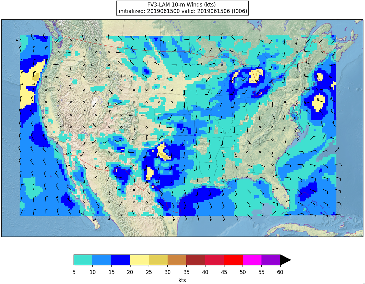
Here is an example plot of 10m surface wind at F006:
Running with batch script
(Estimated time: 25 min wall time for 48 forecast hours, every 3 hours)
There are some batch scripts under the same directory with the python scripts. If the batch script qsub_job.sh is being used to run the plotting script, multiple environment variables need to be set prior to submitting the script besides the python environment:
For bash:
export EXPTDIR=/glade/scratch/$USER/expt_dirs/test_CONUS_25km_GFSv15p2
For csh/tcsh:
setenv EXPTDIR /glade/scratch/$USER/expt_dirs/test_CONUS_25km_GFSv15p2
The HOMErrfs gives the location of regional workflow and EXPTDIR points to the experiment directory (test_CONUS_25km_GFSv15p2). In addition, the account to run the batch job in qsub_job.sh needs to be set. You might wish to change the FCST_INC in the batch script for different plotting frequency, and increase the walltime to 25 minutes (for 48 forecast hours, every 3 hours).
Then the batch job can be submitted by the following command:
qsub qsub_job.sh
The running log will be in the file $HOMErrfs/ush/Python/plot_allvars.out when the job completes.
The output files (in .png format) will be located in the same directory as the command line run: $EXPTDIR/2019061500/postprd
Session 2
Session 2In this session, you will:
- Change the predefined grid resolution
- Change the physics suite and the external models for generating ICs and LBCs
- Define a custom regional ESG grid
1. Changing the Predefined Grid
1. Changing the Predefined GridChanging the Predefined Grid
Starting with the configuration file from Session 1, we will now generate a new experiment that runs a forecast on a CONUS domain with 3km nominal resolution (as opposed to the 25km from Session 1). Since this is only for demonstration purposes, we will also decrease the forecast time from 48 hours to 6 hours. The steps are as follows:
1. For convenience, in your bash shell set SR_WX_APP_TOP_DIR to the path in which you cloned the UFS-SRW App, e.g.
Then set the following variables:
USHDIR="$HOMErrfs/ush"
2. Change location to USHDIR and make a backup copy of your config.sh from the Session 1 experiment:
cp config.sh config.sh.session_1
3. Edit config.sh as follows:
a. Change the name of the experiment directory (which is also the name of the experiment) to something that properly represents the new settings:
b. Change the name of the predefined grid to the CONUS grid with 3km resolution:
c. Change the forecast length to 6 hours:
4. [OPTIONAL] In order to have cron automatically relaunch the workflow without the user having to edit the cron table, add the following lines to the end of (or anywhere in) config.sh:
CRON_RELAUNCH_INTVL_MNTS=03
During the experiment generation step below, these settings will create an entry in the user’s cron table to resubmit the workflow every 3 minutes until either all workflow tasks complete successfully or there is a failure in one of the tasks. (Recall that creation of this cron job was done manually in Session 1.)
5. Generate a new experiment using this configuration file:
a. Ensure that the proper workflow environment is loaded:
b. Generate the workflow:
./generate_FV3LAM_wflow.sh
After this completes, for convenience, in your shell define the variable EXPTDIR to the directory of the experiment created by this script:
EXPTDIR=${SR_WX_APP_TOP_DIR}/../expt_dirs/${EXPT_SUBDIR}
6. If you did not include the parameters USE_CRON_TO_RELAUNCH and CRON_RELAUNCH_INTVL_MNTS in your config.sh (the optional step above), create a cron job to automatically relaunch the workflow as follows:
a. Open your cron table for editing
This will open the cron table for editing (in vi).
b. Insert the following line at the end of the file:
The path to my_expt_name must be edited manually to match the value in EXPTDIR.
7. Monitor the status of the workflow:
rocotostat -w FV3LAM_wflow.xml -d FV3LAM_wflow.db -v 10
Continue to monitor until all workflow tasks complete successfully. Note that the status of the workflow will change only after every 3 minutes because the cron job to relaunch the workflow is called at this frequency.
If you don’t want to wait 3 minutes for the cron job (e.g. because your workflow tasks complete in a much shorter time, which is the case for this experiment), you can relaunch the workflow and update its status yourself at any time by calling the launch_FV3LAM_wflow.sh script from your experiment directory and then checking the log file it appends to. This is done as follows:
./launch_FV3LAM_wflow.sh
tail -n 40 log.launch_FV3LAM_wflow
The launch_FV3LAM_wflow.sh script does the following:
- Issues the rocotorun command to update and relaunch the workflow from its previous state.
- Issues the rocotostat command (same as above) to obtain the table containing the status of the various workflow tasks.
- Checks the output of the rocotostat command for the string “FAILURE” that indicates that at least one task has failed.
- Appends the output of the rocotorun and rocotostat commands to a log file in $EXPTDIR named log.launch_FV3LAM_wflow.
- Counts the number of cycles that have completed successfully.
8. Once all workflow tasks have successfully completed, plot and display the output using a procedure analogous to the one in Session 1 but modified for the shorter forecast time. The steps are:
- Purge all modules and load the one needed for the plotting:
module purge
module load ncarenv
ncar_pylib /glade/p/ral/jntp/UFS_SRW_app/ncar_pylib/python_graphics - Change location to where the python plotting scripts are located:
cd $USHDIR/Python - Call the plotting script. Since this takes some time, here we will plot only the 0th and 6th hour forecasts as follows:
Note: The following is a one-line command.python plot_allvars.py 2019061500 0 6 6 $EXPTDIR /glade/p/ral/jntp/UFS_SRW_app/tools/NaturalEarth -
This takes about 6 minutes to complete. The plots (in png format) will be placed in the directory $EXPTDIR/2019061500/postprd. If you wish, you can generate plots for all forecast hours by changing the second "6" in the call above to a "1", i.e.
Note: The following is a one-line command.python plot_allvars.py 2019061500 0 6 1 $EXPTDIR /glade/p/ral/jntp/UFS_SRW_app/tools/NaturalEarthNote: If you have gone back and forth between experiments in this session, before issuing the python plotting command above, make sure that you have (re)defined EXPTDIR in your shell to the one for the correct experiment. You can check its value usingecho $EXPTDIR - As the plots appear in that directory, if you have an X-windows server running on your local machine, you can display them as follows:
cd $EXPTDIR/2019061500/postprd
display name_of_file.png &where name_of_file.png should be replaced by the name of the file you’d like to display.
2. Changing the SDF and the External Models for Generating ICs and LBCs
2. Changing the SDF and the External Models for Generating ICs and LBCsChanging the Physics Suite and the External Models for Generating ICs and LBCs
Starting with the configuration file created above for the 3km run with the GFS_v15p2 physics suite, we will now generate a new experiment that runs a forecast on the same predefined 3km CONUS grid but uses instead the RRFS_v1alpha physics suite. This will require that we change the external models from which the initial conditions (ICs) and lateral boundary conditions (LBCs) are generated from the FV3GFS (as was the case in the previous experiment) to the HRRR for ICs and the RAP for LBCs because several of the fields needed by the RRFS_v1alpha suite are available in the HRRR and RAP output files but not in those of the FV3GFS. Also, we will demonstrate how to change the frequency with which the lateral boundaries are specified. The steps are as follows:
- Change location to USHDIR and make a backup copy of your config.sh from the experiment in Session 2.1:
cd $USHDIR
cp config.sh config.sh.session_2p1 - Edit config.sh as follows:
- Change the name of the experiment directory to something that properly represents the new experiment:
EXPT_SUBDIR="test_CONUS_3km_RRFS_v1alpha" - Change the name of the physics suite:
CCPP_PHYS_SUITE="FV3_RRFS_v1alpha" - Change the time interval (in hours) with which the lateral boundaries will be specified (using data from the RAP):
LBC_SPEC_INTVL_HRS="3"Note that for the 6-hour forecast we are running here will require two LBC files from the RAP: one for forecast hour 3 and another for hour 6. We specify the names of these files below via the parameter EXTRN_MDL_FILES_LBCS. Note also that the boundary conditions for hour 0 are included in the file for the ICs (from the HRRR). - Change the name of the external model that will provide the fields from which to generate the ICs to the "HRRR", the name of the HRRR file, and the base directory in which it is located:
Note the "X" at the end of the path name.EXTRN_MDL_NAME_ICS="HRRR"
EXTRN_MDL_SOURCE_BASEDIR_ICS="/glade/p/ral/jntp/UFS_SRW_app/staged_extrn_mdl_files/HRRRX"
EXTRN_MDL_FILES_ICS=( "hrrr.out.for_f000" ) - Change the name of the external model that will provide the fields from which to generate the LBCs to "RAP", the names of the RAP files, and the base directory in which they are located:
Note the "X" at the end of the path name.EXTRN_MDL_NAME_LBCS="RAP"
EXTRN_MDL_SOURCE_BASEDIR_LBCS="/glade/p/ral/jntp/UFS_SRW_app/staged_extrn_mdl_files/RAPX"
EXTRN_MDL_FILES_LBCS=( "rap.out.for_f003" "rap.out.for_f006" )The files rap.out.for_f003 and rap.out.for_f006 will be used to generate the LBCs for forecast hours 3 and 6, respectively.
- Change the name of the experiment directory to something that properly represents the new experiment:
- Generate a new experiment using this configuration file:
- Ensure that the proper workflow environment is loaded and generate the experiment directory and corresponding rocoto workflow:
source ../../env/wflow_cheyenne.env
cd $USHDIR
./generate_FV3LAM_wflow.sh - After this completes, for convenience, in your shell redefine the variable EXPTDIR to the directory of the current experiment:
EXPT_SUBDIR="test_CONUS_3km_RRFS_v1alpha"
EXPTDIR="${SR_WX_APP_TOP_DIR}/../expt_dirs/${EXPT_SUBDIR}"
- Ensure that the proper workflow environment is loaded and generate the experiment directory and corresponding rocoto workflow:
- If in Session 2.1 you did not set the parameters USE_CRON_TO_RELAUNCH and CRON_RELAUNCH_INTVL_MNTS in your config.sh, you will have to create a cron job to automatically relaunch the workflow. Do this using the same procedure as in Session 2.1.
- Monitor the status of the workflow:
cd $EXPTDIR
rocotostat -w FV3LAM_wflow.xml -d FV3LAM_wflow.db -v 10Continue to monitor until all the tasks complete successfully. Alternatively, as in Session 2.1, you can use the launch_FV3LAM_wflow.sh script to relaunch the workflow (instead of waiting for the cron job to relaunch it) and obtain its updated status as follows:
cd $EXPTDIR
./launch_FV3LAM_wflow.sh
tail -n 40 log.launch_FV3LAM_wflow - Once all workflow tasks have successfully completed, you can plot and display the output using a procedure analogous to the one described in Session 2.1. Here, we will demonstrate how to generate difference plots between two forecasts on the same grid. The two forecasts we will use are the one in Session 2.1 that uses the GFS_v15p2 suite and the one here that uses the RRFS_v1alpha suite. The steps are:
- Purge all modules and load the one needed for the plotting:
module purge
module load ncarenv
ncar_pylib /glade/p/ral/jntp/UFS_SRW_app/ncar_pylib/python_graphics - Change location to where the python plotting scripts are located:
cd $USHDIR/Python - For convenience, define variables containing the paths to the two forecast experiment directories:
EXPTDIR_2p1=${SR_WX_APP_TOP_DIR}/../expt_dirs/test_CONUS_3km_GFSv15p2
EXPTDIR_2p2=${SR_WX_APP_TOP_DIR}/../expt_dirs/test_CONUS_3km_RRFS_v1alpha - Call the plotting script. Since this takes some time, here we will plot only the 0th and 6th hour differences, as follows:
Note: The following is a one-line command.python plot_allvars_diff.py 2019061500 0 6 6 ${EXPTDIR_2p2} ${EXPTDIR_2p1} /glade/p/ral/jntp/UFS_SRW_app/tools/NaturalEarthThe difference plots (in png format) will be placed under the first experiment directory specified in the call above, which in this case is EXPTDIR_2p2. Thus, the plots will be in ${EXPTDIR_2p2}/2019061500/postprd. (Note that specifying EXPTDIR_2p1 first in the call above would overwrite the plots generated in Session 2.1.) If you wish, you can generate difference plots for all forecast hours by changing the second "6" in the call above to a "1".
- As the difference plots appear in that directory, you can display them as follows:
cd ${EXPTDIR_2p2}/2019061500/postprd
display name_of_file.png &
- Purge all modules and load the one needed for the plotting:
3. Defining a Custom Regional ESG Grid
3. Defining a Custom Regional ESG GridIn this part, we will demonstrate how to define a custom regional ESG (Extended Schmidt Gnomonic) grid instead of using one of the predefined ones. Note that in addition to this grid, we must define a corresponding write-component grid. This is the grid on which the fields are provided in the output files. (This remapping from the native ESG grid to the write-component grid is done because tasks downstream of the forecast may not be able to work with the native grid.)
To define the custom ESG grid and the corresponding write-component grid, three groups of parameters must be added to the experiment configuration file config.sh:
- ESG grid parameters
- Computational parameters
- Write-component grid parameters
Below, we will demonstrate how to add these parameters for a new 3 km sub-CONUS ESG grid. For reference, note that for the predefined grids, these parameters are set in the script $USHDIR/set_predef_grid_params.sh.
First, change location to USHDIR and make a backup copy of your config.sh from the experiment in Session 2.2:
cp config.sh config.sh.session_2p2
For this experiment, we will start with the configuration file used in Session 2.1 and modify it. Thus, first copy it into config.sh:
Now edit config.sh as follows:
- Change the name of the experiment directory to something that properly represents the purpose of this experiment:
EXPT_SUBDIR="test_custom_ESGgrid" - Comment out the line that defines the predefined grid, i.e. change the line
PREDEF_GRID_NAME="RRFS_CONUS_3km"to
#PREDEF_GRID_NAME="RRFS_CONUS_3km" - Ensure that the grid generation method is set to "ESGgrid", i.e. you should see the line
GRID_GEN_METHOD="ESGgrid"right after the line for PREDEF_GRID_NAME that you commented out in the previous step. If not, make sure to include it. The other valid value for this parameter is "GFDLgrid", but we will not demonstrate adding that type of grid here; ESG grids are preferred because they provide more uniform grid size distributions.
- Ensure that QUILTING is set to "TRUE". This tells the experiment to remap output fields from the native ESG grid onto a new orthogonal grid known as the write-component grid and then write the remapped grids to a file using a dedicated set of MPI processes.
- Add the definitions of the ESG grid parameters after the line for QUILTING:
- Define the longitude and latitude (in degrees) of the center of the grid:
ESGgrid_LON_CTR="-114.0"
ESGgrid_LAT_CTR="37.0" - Define the grid cell size (in meters) in the x (west-to-east) and y (south-to-north) directions:
ESGgrid_DELX="3000.0"
ESGgrid_DELY="3000.0" - Define the number of grid cells in the x and y directions:
ESGgrid_NX="420"
ESGgrid_NY="300" - Define the number of halo points around the grid with a “wide” halo
ESGgrid_WIDE_HALO_WIDTH="6"This parameter can always be set to "6" regardless of the other grid parameters.
- Define the longitude and latitude (in degrees) of the center of the grid:
- Add the definitions of computational parameters after the definitions of the ESG grid parameters:
- Define the physics time step (in seconds) to use in the forecast model with this grid:
DT_ATMOS="45"This is the largest time step in the model. It is the time step on which the physics parameterizations are called. In general, DT_ATMOS depends on the horizontal resolution of the grid. The finer the grid, the smaller it needs to be to avoid numerical instabilities.
- Define the MPI layout:
LAYOUT_X="16"
LAYOUT_Y="10"These are the number of MPI processes into which to decompose the grid.
- Define the block size. This is a machine-dependent parameter that does not have a default value. For Cheyenne, set it to "32":
BLOCKSIZE="32"
- Define the physics time step (in seconds) to use in the forecast model with this grid:
- Add the definitions of the write-component grid parameters right after the computational parameters. The workflow supports three types of write-component grids: regional lat-lon, rotated lat-lon, and Lambert conformal. Here, we demonstrate how to set up a Lambert conformal grid. (Note that there are scripts to calculate the write-component grid parameters from the ESG grid parameters, but they are not yet in user-friendly form. Thus, here, we use an approximate method to obtain the write-component parameters.) The steps are:
- Define the number of write-component groups (WRTCMP_write_groups) and the number of MPI processes per group (WRTCMP_write_tasks_per_group):
WRTCMP_write_groups="1"
WRTCMP_write_tasks_per_group=$(( 1*LAYOUT_Y ))Each write group consists of a set of dedicated MPI processes that writes the fields on the write-component grid to a file on disk while the forecast continues to run on a separate set of processes. These parameters may have to be increased for grids having more grid points.
- Define the type of write-component grid. Here, we will consider only a Lambert conformal grid:
WRTCMP_output_grid="lambert_conformal" - Define the longitude and latitude (in degrees) of the center of the write-component grid. The most straightforward way to define these is to set them to the coordinates of the center of the native ESG grid:
WRTCMP_cen_lon="${ESGgrid_LON_CTR}"
WRTCMP_cen_lat="${ESGgrid_LAT_CTR}" - Define the first and second standard latitudes associated with a Lambert conformal coordinate system. For simplicity, we set these to the latitude of the center of the ESG grid:
WRTCMP_stdlat1="${ESGgrid_LAT_CTR}"
WRTCMP_stdlat2="${ESGgrid_LAT_CTR}" - Define the grid cell size (in meters) in the x (west-to-east) and y (south-to-north) directions on the write-component grid. We simply set these to the corresponding quantities for the ESG grid:
WRTCMP_dx="${ESGgrid_DELX}"
WRTCMP_dy="${ESGgrid_DELY}" - Define the number of grid points in the x and y directions on the write-component grid. To ensure that the write-component grid lies completely within the ESG grid, we set these to 95% of ESGgrid_NX and ESGgrid_NY, respectively. This gives
WRTCMP_nx="399"
WRTCMP_ny="285" - Define the longitude and latitude (in degrees) of the lower left (southwest) corner of the write-component grid. Approximate values (from a linearization that is more accurate the smaller the horizontal extent of the grid) for these quantities can be obtained using the formulas (for reference):
WRTCMP_lon_lwr_left = WRTCMP_cen_lon - (degs_per_meter/(2*cos_phi_ctr))*WRTCMP_nx*WRTCMP_dx
WRTCMP_lat_lwr_left = WRTCMP_cen_lat - (degs_per_meter/2)*WRTCMP_ny*WRTCMP_dywhere
cos_phi_ctr = cos((180/pi_geom)*WRTCMP_lat_lwr_left)
degs_per_meter = 180/(pi_geom*radius_Earth)Here, pi_geom ≈ 3.14 and radius_Earth ≈ 6371e+3 m. Substituting in these values along with the write-component grid parameters set above, we get
WRTCMP_lon_lwr_left="-120.74"
WRTCMP_lat_lwr_left="33.16"
- Define the number of write-component groups (WRTCMP_write_groups) and the number of MPI processes per group (WRTCMP_write_tasks_per_group):
For simplicity, we leave all other parameters in config.sh the same as in the experiment in Session 2.1. We can now generate a new experiment using this configuration file as follows:
- Ensure that the proper workflow environment is loaded and generate the experiment directory and corresponding rocoto workflow:
source ../../env/wflow_cheyenne.env
cd $USHDIR
./generate_FV3LAM_wflow.sh - After this completes, for convenience, in your shell redefine the variable EXPTDIR to the directory of the current experiment:
EXPT_SUBDIR="test_custom_ESGgrid"
EXPTDIR="${SR_WX_APP_TOP_DIR}/../expt_dirs/${EXPT_SUBDIR}" - Relaunch the workflow using the launch_FV3LAM_wflow.sh script and monitor its status:
cd $EXPTDIR
./launch_FV3LAM_wflow.sh
tail -n 80 log.launch_FV3LAM_wflow - Once all workflow tasks have successfully completed, plot and display the output using a procedure analogous to the one in Session 2.1. (Before doing so, make sure that the shell variable EXPTDIR is set to the directory for this experiment; otherwise, you might end up generating plots for one of the other experiments!)
Session 3
Session 3In this session you will:
- Customize the Unified Post Processor (UPP) output by adding/removing fields/levels in the GRIB2 SRW App output files
- Change a physics scheme in an existing Suite Definition File (SDF)
1. Customizing Unified Post Processor (UPP) Output
1. Customizing Unified Post Processor (UPP) OutputThe following set of instructions will guide you through how to customize the UPP configuration file to add/remove fields/levels in the Grib2 output for SRW v1.0.1. This requires a pre-processing step to create the flat text configuration file that UPP reads. This guide assumes you have already completed Session 1: Setup and Run the Workflow.
- Set environment variables as was done in Session 1:
SCRATCH_DIR=/glade/scratch/$USER
SR_WX_APP_TOP_DIR=$SCRATCH_DIR/ufs-srweather-app
EXPT_SUBDIR=test_CONUS_25km_GFSv15p2
EXPTDIR=${SR_WX_APP_TOP_DIR}/../expt_dirs/${EXPT_SUBDIR} - Move to the directory that contains the configuration files and scripts used for creating a custom flat text file read by UPP.
cd ${SR_WX_APP_TOP_DIR}/src/EMC_post/parm - Create a copy of the original fv3lam.xml file that will be modified so you do not overwrite the original. This is the file that lists all variables you would like to output.
cp fv3lam.xml fv3lam.xml.${USER}For a complete list of fields that can be output by UPP, please refer to the UPP Grib2 table in the online documentation. (Please note that some fields can only be output using certain models and/or physics options.)
- Example 1: Adding a simple field
This example describes how to add the field POT (potential temperature) on pressure levels to the fv3lam.xml.${USER} configuration file. This configuration file is split into two sections; BGDAWP and BGRD3D. Edit the configuration file by adding the following parameter to the BGRD3D section (search BGRD3D), but before the </paramset> tag at the bottom of the file.<param>
<shortname>POT_ON_ISOBARIC_SFC</shortname>
<pname>POT</pname>
<level>25000. 50000. 70000. 85000.</level>
<scale>4.0</scale>
</param>You may also delete an unwanted field by completely removing the parameter block of that field from the XML file and then continuing with step 7.
* Formatting is important; use other entries in the file as a guide.
** Adding fields requires knowledge on which fields can be output for your specific dynamic core and physics options. Not all fields available in UPP can be output with the UFS SRW application.
- Example 2: Adding levels to a field
This example will describe how to add levels to a field in the fv3lam.xml.${USER} configuration file. Edit the configuration file by adding the bold highlighted levels (in geopotential meters) to the field ‘Specific humidity on flight levels’.<param>
<shortname>SPFH_ON_SPEC_HGT_LVL_ABOVE_GRND_FDHGT</shortname>
<level>20. 30. 40. 50. 80. 100. 305. 610. 1524.</level>
<scale>4.0</scale>
</param>For the list of available levels for each level type, please reference the UPP documentation on ‘Controlling which levels UPP outputs’. You may also easily remove levels from the tag by simply deleting them from the list.
- Example 3: Adding a satellite brightness temperature field
This example describes how to add the field SBTA169 (GOES-16 Channel 9; IR mid-level troposphere water vapor) to the fv3lam.xml.${USER} configuration file. (Note that while other channels are available for GOES-16, we are only adding this one).
Edit the configuration file by adding the following parameter to the BGDAWP section, but before the </paramset> tag (~L1820 of the original file).<param>
<shortname>SBTA169_ON_TOP_OF_ATMOS</shortname>
<scale>4.0</scale>
</param>In order to output a satellite brightness temperature field, the CRTM coefficient files for each of the satellites are needed. Move to the top level UPP directory, pull the CRTM fix tar file, and unpack.
cd ${SR_WX_APP_TOP_DIR}/src/EMC_post/
mkdir crtm && cd crtm
wget https://github.com/NOAA-EMC/EMC_post/releases/download/upp_v9.0.0/fix.tar.gz
tar -xzf fix.tar.gzThese coefficient files need to be copied to the UPP working directory and to do so requires modification of the UPP run script. Edit the file ${SR_WX_APP_TOP_DIR}/regional_workflow/scripts/exregional_run_post.sh to add the following lines in the same location where other files are being copied to the UPP run directory (~L189).
# Copy coefficients for crtm2 (simulated synthetic satellites)
cp_vrfy ${EMC_POST_DIR}/crtm/fix/EmisCoeff/IR_Water/Big_Endian/Nalli.IRwater.EmisCoeff.bin ./
cp_vrfy ${EMC_POST_DIR}/crtm/fix/EmisCoeff/MW_Water/Big_Endian/FAST*.bin ./
cp_vrfy ${EMC_POST_DIR}/crtm/fix/EmisCoeff/IR_Land/SEcategory/Big_Endian/NPOESS.IRland.EmisCoeff.bin ./
cp_vrfy ${EMC_POST_DIR}/crtm/fix/EmisCoeff/IR_Snow/SEcategory/Big_Endian/NPOESS.IRsnow.EmisCoeff.bin ./
cp_vrfy ${EMC_POST_DIR}/crtm/fix/EmisCoeff/IR_Ice/SEcategory/Big_Endian/NPOESS.IRice.EmisCoeff.bin ./
cp_vrfy ${EMC_POST_DIR}/crtm/fix/AerosolCoeff/Big_Endian/AerosolCoeff.bin ./
cp_vrfy ${EMC_POST_DIR}/crtm/fix/CloudCoeff/Big_Endian/CloudCoeff.bin ./
cp_vrfy ${EMC_POST_DIR}/crtm/fix/SpcCoeff/Big_Endian/*.bin ./
cp_vrfy ${EMC_POST_DIR}/crtm/fix/TauCoeff/ODPS/Big_Endian/*.bin ./ - In order to ensure there are no errors in your modified fv3lam.xml.${USER} file, you may validate it against the XML stylesheets provided in the UPP parm directory.
cd ${SR_WX_APP_TOP_DIR}/src/EMC_post/parm
xmllint --noout --schema EMC_POST_CTRL_Schema.xsd fv3lam.xml.${USER}If the XML is error free, then the command will return that the XML validates. (e.g. fv3lam.xml.${USER} validates)
- Create the flat text file.
Note: The following is a one-line command./usr/bin/perl PostXMLPreprocessor.pl fv3lam.xml.${USER} fv3lam_post_avblflds.xml postxconfig-NT-fv3lam.txt.${USER}The perl program PostXMLPreprocessor.pl processes the modified xml and creates the flat text configuration file with the file name provided. In this case the new flat text file is postxconfig-NT-fv3lam.txt.${USER} and should now exist in the parm directory if this step was successful.
- To run the SRW post-processing with this new customized flat text file for the experiment from session 1, move back to the directory with the workflow configuration file.
cd ${SR_WX_APP_TOP_DIR}/regional_workflow/ushCopy the config file from session 1 back to config.sh.
cp config.sh.session_1 config.shThen modify the config.sh, adding the following lines:
USE_CUSTOM_POST_CONFIG_FILE="TRUE"
CUSTOM_POST_CONFIG_FP="/glade/scratch/${USER}/ufs-srweather-app/src/EMC_post/parm/postxconfig-NT-fv3lam.txt.${USER}"Setting the USE_CUSTOM_POST_CONFIG_FILE to TRUE tells the workflow to use the custom file located in the user-defined path, CUSTOM_POST_CONFIG_FP. The path should include the filename. If this is set to true and the file path is not found, then an error will occur when trying to generate the SRW Application workflow using the generate_FV3LAM_wflow.sh script.
- You can then proceed with running the workflow using the modified configuration file.
Load the Python environment and generate the FV3LAM workflow.
source ${SR_WX_APP_TOP_DIR}/env/wflow_cheyenne.env
./generate_FV3LAM_wflow.shStart the entire case workflow following the instructions from Session 1: Step 4. Run the Workflow and UPP will use the new flat postxconfig-NT-fv3lam.txt.${USER} file. Once the workflow is complete, the new UPP output should include the added fields and levels.
Optional Downstream Application examples for UPP output
You can check the contents of the UPP output using a simple wgrib2 command. Move to the directory containing the UPP output.
Load the module for wgrib2 on Cheyenne and use it to list the fields within the Grib2 files.
wgrib2 rrfs.t00z.bgdawpf036.tm00.grib2
wgrib2 rrfs.t00z.bgrd3df036.tm00.grib2
Or for additional diagnostic output such as min/max values and grid specs:
wgrib2 -V rrfs.t00z.bgrd3df036.tm00.grib2
If you want to seach for a specific variable rather than printing out the entire list:
You can produce a simple plot of the GOES-16, channel 9 field that we added in step 6 using the Model Evaluation Tools (MET) plot_data_plane function.
Load METv10.0.0 via a module on Cheyenne.
module load met/10.0.0
In the postprd directory, use the plot_data_plane tool to create a postscript file.
gv SBTA169_2019061500_f036.ps
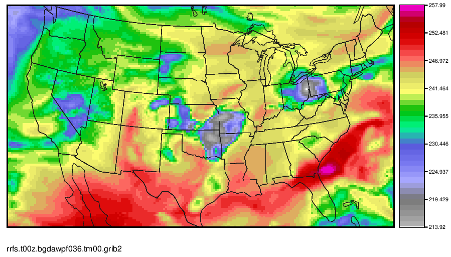
The GOES-16 Channel 9 (IR mid-level troposphere water vapor) image at F036 should look like this.
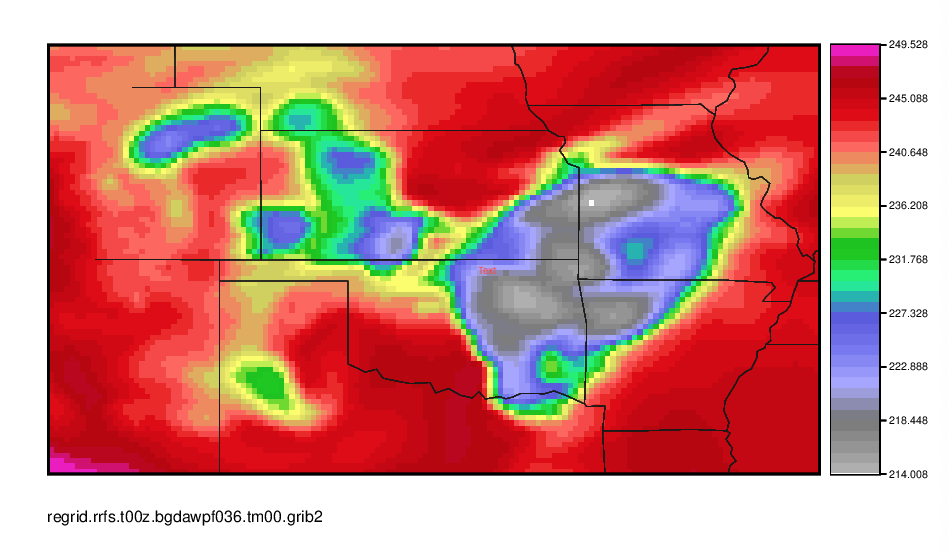
Regrid UPP output using wgrib2 and create a simple plot using MET. (Note that MET also has regrid capabilities; however, for those without the MET software, wgrib2 is a great tool)
UPP grib2 output is on the same grid as the model output, which for this SRW case is a 25 km Lambert Conformal grid. This example shows how to transform to a lat-lon grid. The specifications for a simple lat-lon projection are:
| Variable | Description |
|---|---|
| lon0/lat0 | Longitude/Latitude of first grid point in degrees |
| nlon/nlat | Number of Longitudes/Latitudes |
| dlon/dlat | Grid resolution in degrees of Longitude/Latitude |
Example:
This will interpolate to a 0.125 degree latitude-longitude grid with earth-relative winds (U-wind goes east, V-wind goes north), zoomed in on the region of active convection.
Make a quick plot of GOES-16 Channel 9 from the newly regrid data using MET.
gv SBTA169_2019061500_f036_regrid.ps
You can also view the contents of the new file with wgrib2 as before.
For more wgrib2 options/examples, you can refer to the wgrib2 site.
For more information on MET/METplus, refer to the MET Users Page/METplus Users Page.
2. Changing a Physics Scheme in the Suite Definition File (SDF)
2. Changing a Physics Scheme in the Suite Definition File (SDF)The following set of instructions will guide you through the process of changing the land surface model from Noah to NoahMP in the suite GFSv15p2.
- Go to the suite definition file directory:
The physics schemes for the GFSv15p2 suite are defined in the suite definition file suite_FV3_GFS_v15p2.xml under the directory: /glade/scratch/$USER/ufs-srweather-app/src/ufs_weather_model/FV3/ccpp/suites
Change to the suite directory and check the suite files:cd /glade/scratch/$USER/ufs-srweather-app/src/ufs_weather_model/FV3/ccpp/suites
ls -1suite_FV3_GFS_v15p2.xml
suite_FV3_RRFS_v1alpha.xml
suite.xsdThe suite definition file is a text file, and a modified suite can be constructed from the existing SDF. A modified suite can be constructed from an existing SDF through copying the existing suite file and changing other aspects of the file.
cp suite_FV3_GFS_v15p2.xml suite_FV3_GFS_v15p2_noahmp.xml - Modify the GFSv15p2_noahmp SDF file with a new land surface model(LSM):
- To change the Noah land surface model (lsm_noah) to noah_mp land surface model (noahmpdrv) in suite_FV3_GFS_v15p2_noahmp.xml, change:
<scheme>lsm_noah</scheme>to
<scheme>noahmpdrv</scheme> - Change the suite name in the file from:
<suite name="FV3_GFS_v15p2" lib="ccppphys" ver="5">to
<suite name="FV3_GFS_v15p2_noahmp" lib="ccppphys" ver="5">
- To change the Noah land surface model (lsm_noah) to noah_mp land surface model (noahmpdrv) in suite_FV3_GFS_v15p2_noahmp.xml, change:
- Add the new suite to the compiling command:
Edit the file /glade/scratch/$USER/ufs-srweather-app/src/CMakeLists.txt by changing:set(CCPP_SUITES "FV3_GFS_v15p2,FV3_RRFS_v1alpha")to
set(CCPP_SUITES "FV3_GFS_v15p2,FV3_GFS_v15p2_noahmp,FV3_RRFS_v1alpha")so the new suite is included in the compiling of the model.
- Modify the Workflow to include the new suite:
- Add suite FV3_GFS_v15p2_noahmp to the file FV3.input.yml under the directory /glade/scratch/$USER/ufs-srweather-app/regional_workflow/ush/templates. Insert the following part after line 272 in FV3.input.yml:
FV3_GFS_v15p2_noahmp:
atmos_model_nml:
fdiag: 1
fms_nml:
domains_stack_size: 1800200
fv_core_nml:
<<: *gfs_v15_fv_core
agrid_vel_rst: False
d2_bg_k1: 0.15
d2_bg_k2: 0.02
dnats: 1
do_sat_adj: True
fv_debug: False
fv_sg_adj: 600
k_split: 1
kord_mt: 9
kord_tm: -9
kord_tr: 9
kord_wz: 9
n_split: 8
n_sponge: 30
nord_zs_filter: !!python/none
nudge_qv: True
range_warn: False
rf_cutoff: 750.0
rf_fast: False
gfdl_cloud_microphysics_nml:
<<: *gfs_gfdl_cloud_mp
sedi_transport: True
tau_l2v: 225.0
tau_v2l: 150.0
gfs_physics_nml:
<<: *gfs_v15_gfs_physics
bl_mynn_edmf: !!python/none
bl_mynn_edmf_mom: !!python/none
bl_mynn_tkeadvect: !!python/none
cnvcld: True
cnvgwd: True
cplflx: !!python/none
do_myjpbl: False
do_myjsfc: False
do_mynnedmf: !!python/none
do_mynnsfclay: !!python/none
do_tofd: False
do_ugwp: False
do_ysu: False
fhcyc: 0.0
fhlwr: 3600.0
fhswr: 3600.0
fhzero: 6.0
hybedmf: True
iau_delthrs: !!python/none
iaufhrs: !!python/none
imfdeepcnv: 2
imfshalcnv: 2
imp_physics: 11
icloud_bl: !!python/none
iopt_alb: 2
iopt_btr: 1
iopt_crs: 1
iopt_dveg: 2
iopt_frz: 1
iopt_inf: 1
iopt_rad: 1
iopt_run: 1
iopt_sfc: 1
iopt_snf: 4
iopt_stc: 1
iopt_tbot: 2
ldiag_ugwp: False
lgfdlmprad: True
lradar: !!python/none
lsm: 2
lsoil: !!python/none
lsoil_lsm: !!python/none
ltaerosol: !!python/none
shal_cnv: True
shinhong: False
ttendlim: !!python/none
xkzm_h: 1.0
xkzm_m: 1.0
xkzminv: 0.3
namsfc:
landice: True
ldebug: False
surf_map_nml:It’s similar to the setting for suite FV3_GFS_v15p2 except the lsm=2.
- Prepare tables for noahmp:
cp field_table.FV3_GFS_v15p2 field_table.FV3_GFS_v15p2_noahmp
cp diag_table.FV3_GFS_v15p2 diag_table.FV3_GFS_v15p2_noahmp - Add suite FV3_GFS_v15p2_noahmp to valid_param_vals.sh under /glade/scratch/$USER/ufs-srweather-app/regional_workflow/ush, by changing:
valid_vals_CCPP_PHYS_SUITE=( \
"FV3_GFS_v15p2" \
"FV3_RRFS_v1alpha" \
)to
valid_vals_CCPP_PHYS_SUITE=( \
"FV3_GFS_v15p2" \
"FV3_GFS_v15p2_noahmp" \
"FV3_RRFS_v1alpha" \
) - Add suite FV3_GFS_v15p2_noahmp to files exregional_make_ics.sh, and exregional_make_lbcs.sh under the directory /glade/scratch/$USER/ufs-srweather-app/regional_workflow/scripts:
cd /glade/scratch/$USER/ufs-srweather-app/regional_workflow/scriptsEdit files exregional_make_ics.sh, and exregional_make_lbcs.sh, changing all
[ "${CCPP_PHYS_SUITE}" = "FV3_GFS_v15p2" ] || \to
[ "${CCPP_PHYS_SUITE}" = "FV3_GFS_v15p2" ] || \
[ "${CCPP_PHYS_SUITE}" = "FV3_GFS_v15p2_noahmp" ] || \and changing
"FV3_GFS_v15p2" | "FV3_CPT_v0" )to
"FV3_GFS_v15p2_noahmp" | \
"FV3_GFS_v15p2" | "FV3_CPT_v0" )To confirm the changes, run:
less *.sh | grep v15to get the following messages to make sure the suite is added correctly:
"FV3_GFS_v15p2_noahmp" | \
"FV3_GFS_v15p2" | "FV3_CPT_v0" )
[ "${CCPP_PHYS_SUITE}" = "FV3_GFS_v15p2" ] || \
[ "${CCPP_PHYS_SUITE}" = "FV3_GFS_v15p2_noahmp" ] || \
[ "${CCPP_PHYS_SUITE}" = "FV3_GFS_v15p2" ] || \
[ "${CCPP_PHYS_SUITE}" = "FV3_GFS_v15p2_noahmp" ] || \
[ "${CCPP_PHYS_SUITE}" = "FV3_GFS_v15p2" ] || \
[ "${CCPP_PHYS_SUITE}" = "FV3_GFS_v15p2_noahmp" ] || \
[ "${CCPP_PHYS_SUITE}" = "FV3_GFS_v15p2" ] || \
[ "${CCPP_PHYS_SUITE}" = "FV3_GFS_v15p2_noahmp" ] || \
[ "${CCPP_PHYS_SUITE}" = "FV3_GFS_v15p2" ] || \
[ "${CCPP_PHYS_SUITE}" = "FV3_GFS_v15p2_noahmp" ] || \
"FV3_GFS_v15p2_noahmp" | \
"FV3_GFS_v15p2" | "FV3_CPT_v0" )
[ "${CCPP_PHYS_SUITE}" = "FV3_GFS_v15p2" ] || \
[ "${CCPP_PHYS_SUITE}" = "FV3_GFS_v15p2_noahmp" ] || \
[ "${CCPP_PHYS_SUITE}" = "FV3_GFS_v15p2" ] || \
[ "${CCPP_PHYS_SUITE}" = "FV3_GFS_v15p2_noahmp" ] || \
[ "${CCPP_PHYS_SUITE}" = "FV3_GFS_v15p2" ] || \
[ "${CCPP_PHYS_SUITE}" = "FV3_GFS_v15p2_noahmp" ] || \
- Add suite FV3_GFS_v15p2_noahmp to the file FV3.input.yml under the directory /glade/scratch/$USER/ufs-srweather-app/regional_workflow/ush/templates. Insert the following part after line 272 in FV3.input.yml:
- Compile the model with the new suite:
Users can refer to Session 1 for additional information:cd /glade/scratch/$USER/ufs-srweather-app/
source env/build_cheyenne_intel.env -
mkdir build
cd buildRun cmake to set up the Makefile, then run make:
cmake .. -DCMAKE_INSTALL_PREFIX=..
make -j 4 >& build.out & - Set the config.sh file:
Go to the the ush directorycd /glade/scratch/$USER/ufs-srweather-app/regional_workflow/ush/Use the config.sh from Session 1 and edit the config.sh, making sure the machine and account are set correctly:
MACHINE="cheyenne"
ACCOUNT="NJNT0008"- Change the name of the experiment directory (which is also the name of the experiment) to something that properly represents the new settings:
EXPT_SUBDIR="test_CONUS_25km_GFSv15p2_noahmp" - Set the predefined grid to the CONUS grid with 25km resolution:
PREDEF_GRID_NAME="RRFS_CONUS_25km" - Change the forecast length to 6 hours:
FCST_LEN_HRS="6"Only a 6 hour forecast is used for practice purposes.
- Set the suite:
CCPP_PHYS_SUITE="FV3_GFS_v15p2_noahmp" - Make sure the LBCS and ICS directories are set correctly:
USE_USER_STAGED_EXTRN_FILES="TRUE"
EXTRN_MDL_SOURCE_BASEDIR_ICS="/glade/p/ral/jntp/UFS_SRW_app/staged_extrn_mdl_files/FV3GFS"
EXTRN_MDL_SOURCE_BASEDIR_LBCS="/glade/p/ral/jntp/UFS_SRW_app/staged_extrn_mdl_files/FV3GFS"
- Change the name of the experiment directory (which is also the name of the experiment) to something that properly represents the new settings:
- Generate the workflow with the modified suite file:
Load the appropriate Python environment for Cheyenne:source ../../env/wflow_cheyenne.envGenerate the workflow with the command:
./generate_FV3LAM_wflow.sh - Run the workflow:
- Run the model manually:
cd /glade/scratch/$USER/expt_dirs/test_CONUS_25km_GFSv15p2_noahmp
./launch_FV3LAM_wflow.shThis command needs to be repeated until all the jobs are finished.
- Run the model through the crontab:
For automatic resubmission of the workflow (e.g., every 3 minutes), the following line can be added to the user’s crontab:crontab -eand insert the line:
*/3 * * * * cd /glade/scratch/$USER/expt_dirs/test_CONUS_25km_GFSv15p2_noahmp && ./launch_FV3LAM_wflow.sh
- Run the model manually:
- Check the model running status:
rocotostat -w FV3LAM_wflow.xml -d FV3LAM_wflow.db -v 10The workflow run is completed when all tasks have “SUCCEEDED”
- Generate the plots:
- Change to the python script directory:
cd /glade/scratch/$USER/ufs-srweather-app/regional_workflow/ush/Python - Load the appropriate Python environment for Cheyenne:
module purge
module load ncarenv
ncar_pylib /glade/p/ral/jntp/UFS_SRW_app/ncar_pylib/python_graphicsIf you see something like:
Warning: library /glade/p/ral/jntp/UFS_SRW_app/ncar_pylib/regional_workflow is missing from NPL clone registry.
Do you wish to add it to the registry (y/N)?This will occur if this is the first time you have used the NCAR Python Library (NPL), type ‘y’, to get the following output:
Searching library for configuration info ...
Now using NPL virtual environment at path:
/glade/p/ral/jntp/UFS_SRW_app/ncar_pylib/regional_workflow
Use deactivate to remove NPL from environment - Run the python plotting script:
Note: The following is a one-line command:python plot_allvars.py 2019061500 6 6 6 /glade/scratch/$USER/expt_dirs/test_CONUS_25km_GFSv15p2_noahmp /glade/p/ral/jntp/UFS_SRW_app/tools/NaturalEarth - Display the output figures:
The output files (in .png format) can be found in the directory /glade/scratch/$USER/expt_dirs/test_CONUS_25km_GFSv15p2_noahmp/2019061500/postprdcd /glade/scratch/$USER/expt_dirs/test_CONUS_25km_GFSv15p2_noahmp/2019061500/postprd
display 10mwind_conus_f006.png
- Change to the python script directory:
