CCPP and SCM Online Tutorial
CCPP and SCM Online Tutorial
Welcome to the CCPP and SCM online tutorial.
The goal of this tutorial is to familiarize beginners to the Common Community Physics Package (CCPP) with its key concepts: 1) how it is used within host models, 2) what makes a piece of code compatible with the CCPP, and 3) how collections of physics parameterizations are organized into suites. It includes lecture-like content followed by hands-on exercises. The exercises will be conducted within the context of the CCPP Single Column Model (SCM), so users will also get an introduction to how this model can be used for both science and physics development.
You may navigate through this tutorial by following the links at the bottom of each page or by using the menu navigation on the right hand side.
Each section builds on the output of previous sections. So please work on them in the order listed. If you have questions, please refer to the SCM v7.0.0 User and Technical Guide. If you need additional help, please post a question to the GitHub Discussions.
Throughout this tutorial, code blocks in BOLD white text with a black background should be copied from your browser and pasted on the command line.
echo "Let's Get Started"
To begin, watch the video presentations, by clicking on "Video Presentations" at the bottom (or right).
Video presentations
Video presentations
Video Presentations
Begin this tutorial by viewing the following video presentations:
- CCPP overview presentation
- ~35 minutes of narrated slides to cover CCPP key concepts and capabilities
- YouTube video
- PDF of slides
- SCM overview presentation
- ~15 minutes of narrated slides to cover SCM key concepts and capabilities
- YouTube video
- PDF of slides
Download and Build
Download and Build
Download and Build
Defining your workspace
The first step is to create an environment variable that contains the path to the directory in which you will build and run the SCM.
Go to the directory in which you will build and run the SCM and run the command below substituting /path/to/my/build/and/run/directory with your actual directory name
cd /path/to/my/build/and/run/directory
Next, define an environment variable that contains the path
For bash (Bourne Shell), k:
export SCM_WORK=`pwd`
For C-Shell:
setenv SCM_WORK `pwd`
Download the Tutorial Files
Files that are used throughout the exercises in this tutorial are available to download. Down load these to the $SCM_WORK directory.
wget https://github.com/NCAR/ccpp-scm/releases/download/v7.0.0/tutorial_files.tar.gz
tar -xvf tutorial_files.tar.gz
rm -f tutorial_files.tar.gz
curl -OL https://github.com/NCAR/ccpp-scm/releases/download/v7.0.0/tutorial_files.tar.gzDetermining how you will use the SCM
There are two supported ways to build and run the Single Column Model: the standard build, and with a Docker container. Please follow one of the options below for information on these two methods:
Option 1 Using a pre-configured platform
Option 1 Using a pre-configured platform
Option 1. Using a computational platform with the required software stack
The SCM can build on most modern UNIX-based operating systems, including both MacOS and Linux. It has a few prerequisite libraries and software, including a Fortran compiler compatible with the FORTRAN-08 standard, Python version 3.8 or later, CMake version 3.14 or later, and a few external libraries which may need to be installed:
- NetCDF-c/NetCDF-FORTRAN
- NCEP libraries BACIO, SP, and W3EMC
- Python modules f90nml and netcdf4
This tutorial will assume that you already have these prerequisites installed. Machines that already have the prerequisite software include:
- NCAR Derecho
- NOAA Hera, Jet
- MSU Orion, Hercules
For more details on software prerequisites, including instructions for building on a custom platform, see the SCM Users Guide.
Obtaining the code
The source code for the CCPP and SCM is provided through GitHub.com. This tutorial accompanies the v7.0.0 release tag, which contains the tested and supported version for general use.
Clone the the v7 release code using
git clone --recursive -b release/public-v7 https://github.com/NCAR/ccpp-scm
The recursive option in this command clones the release/public-v7 branch of the NCAR authoritative SCM repository (ccpp-scm) and all submodules/sub-repositories (ccpp-physics, ccpp-framework, and CMakeModules).
Setting up the environment in a preconfigured platform
If using a preconfigured platform, it may be necessary to run on a compute node.
On Hera:
On Derecho:
qinteractive
Computational platforms that meet the system requirements and have the prerequisite software prebuilt and installed in a central location are referred to as preconfigured platforms. Examples of preconfigured platforms are the Hera NOAA high-performance computing machine and the NCAR Derecho system (using the Intel and GNU compilers). The SCM repository contains modulefiles for all pre-configured platforms that can be loaded to set up the environment as needed. These modules set up the needed environment variables, particularly $PATH, so that the SCM will build correctly.
To load the needed module, ensure you are in the top-level ccpp-scm directory, and run the following commands:
module use scm/etc/modules/
module load [machine]_[compiler]
The last command will depend on which machine you are on and what compiler you are using. For example on the NCAR Derecho machine for GNU compilers:
Setting up the environment in a non-preconfigured platform
If you are not using a preconfigured platform, you need to install spack-stack yourself following the instructions found in Section 4.2.4 of the CCPP SCM User and Technical Guide v7-0-0.
After performing the installation and setting environment variables bacio_ROOT, sp_ROOT, and w3nco_ROOT to the location where spack-stack is installed, continue following the instructions in this tutorial.
Staging additional datasets
You need to download the lookup tables (large binaries, 324 MB) for the Thompson microphysics package, the GOCART climatological aerosols, and other datasets. The aerosol data is very large (~12 GB) and is needed when the first digit of the aerosol flag (iaer) in the physics namelist is =1, e.g. GFS_v17_p8_ugwpv1 and HRRR_gf suites.
./contrib/get_all_static_data.sh
./contrib/get_thompson_tables.sh
./contrib/get_aerosol_climo.sh
Building the code
Following the commands below, you will run cmake to query system parameters, execute the CCPP pre-build script to match the physics variables (between what the host model – SCM – can provide and what is needed by physics schemes in the CCPP), and build the physics caps needed to use them. Subsequently, you will run make to build the SCM executable.
mkdir -p bin && cd bin
cmake ../src
make -j4
A successful build will produce the executable file $SCM_WORK/ccpp-scm/scm/bin/scm
Option 2 Using a Docker Container
Option 2 Using a Docker Container
Option 2. Using a Docker container
In order to run a precompiled version of the CCPP SCM in a container, Docker needs to be available on your machine. Please visit https://www.docker.com to download and install the version compatible with your system. Docker frequently releases updates to the software; it is recommended to apply all available updates. NOTE: In order to install Docker on your machine, you need to have root access privileges. More information about getting started can be found at https://docs.docker.com/get-started and in Section 4.5 of the CCPP SCM User and Technical Guide.
In the first exercise you will use a prebuilt Docker image available on Docker Hub. In subsequent exercises you will use the same image to rebuild your own SCM executable with various modifications.
Using a prebuilt Docker image
A prebuilt Docker image is available on Docker Hub. In order to use this, execute the following from the terminal where Docker is run:
To verify that it exists afterward, run the command:
Proceed to “Set up the Docker image”.
Set up the Docker image
Next, you will set up an output directory so that output generated by the SCM and its scripts within the container can be used outside of the container using the following steps:
- Set up a directory that will be shared between the host machine and the Docker container. When set up correctly, it will contain output generated by the SCM within the container for manipulation by the host machine. For Mac/Linux,
For Windows, you can try to create a directory of your choice to mount to the container, but it may not work or may require more configuration, depending on your particular Docker installation. We have found that Docker volume mounting in Windows can be difficult to set up correctly. One method that worked for us was to create a new directory under our local user space, and specify the volume mount as below.
In addition, with Docker Toolbox, double check that the mounted directory has correct permissions. For example, open VirtualBox, right click on the
running virtual machine, and choose “Settings”. In the dialog that appears, make sure that the directory you’re trying to share shows up in “Shared Folders" (and add it if it does not) and make sure that the “auto-mount" and “permanent" options are checked.
- Set an environment variable to point to the directory that was set up in the previous step.
- To use the SCM in the container interactively, run non-default configurations, create plots, or even develop code, issue the following command:
Note that this command will not actually run the SCM, but will put you within the container space and within the bin directory of the SCM with a pre-compiled executable. At this point, you can run the scripts as described in the following sections.
A couple things to note when using a container:
- The run scripts should be used with the -d option if output is to be shared with the host machine
- Since the container is ephemeral, if you do development you should push your changes to a remote git repository to save them (i.e. a fork on GitHub.com).
Exercise 1: Run the SCM and examine the results
Exercise 1: Run the SCM and examine the results
Review the physics suites
You will run two experiments with the SCM, showing the differences between all supported physics suites for a given case based on the Tropical Warm Pool – International Cloud Experiment (TWP-ICE) field campaign. Let’s first take a look at the composition of the physics suites and then at how the case is set up.
Navigate to the directory where the Suite Definition Files (SDFs) are stored and see what is available:
ls
Peruse the files and notice the XML format, paying attention to the key elements: suite (with name attribute), group, subcycle, scheme.
You will find primary and interstitial schemes. All suites share many common elements, including interstitial schemes that are required to prepare data for schemes and calculate diagnostics.
As an example, the differences between the GFS_v16 suite (an approximation of the physics used for the GFS version 16 release) and the WoFS_v0 suite (a prototype for the operational implementation of NOAA's Warn-on-Forecast System) is shown below.
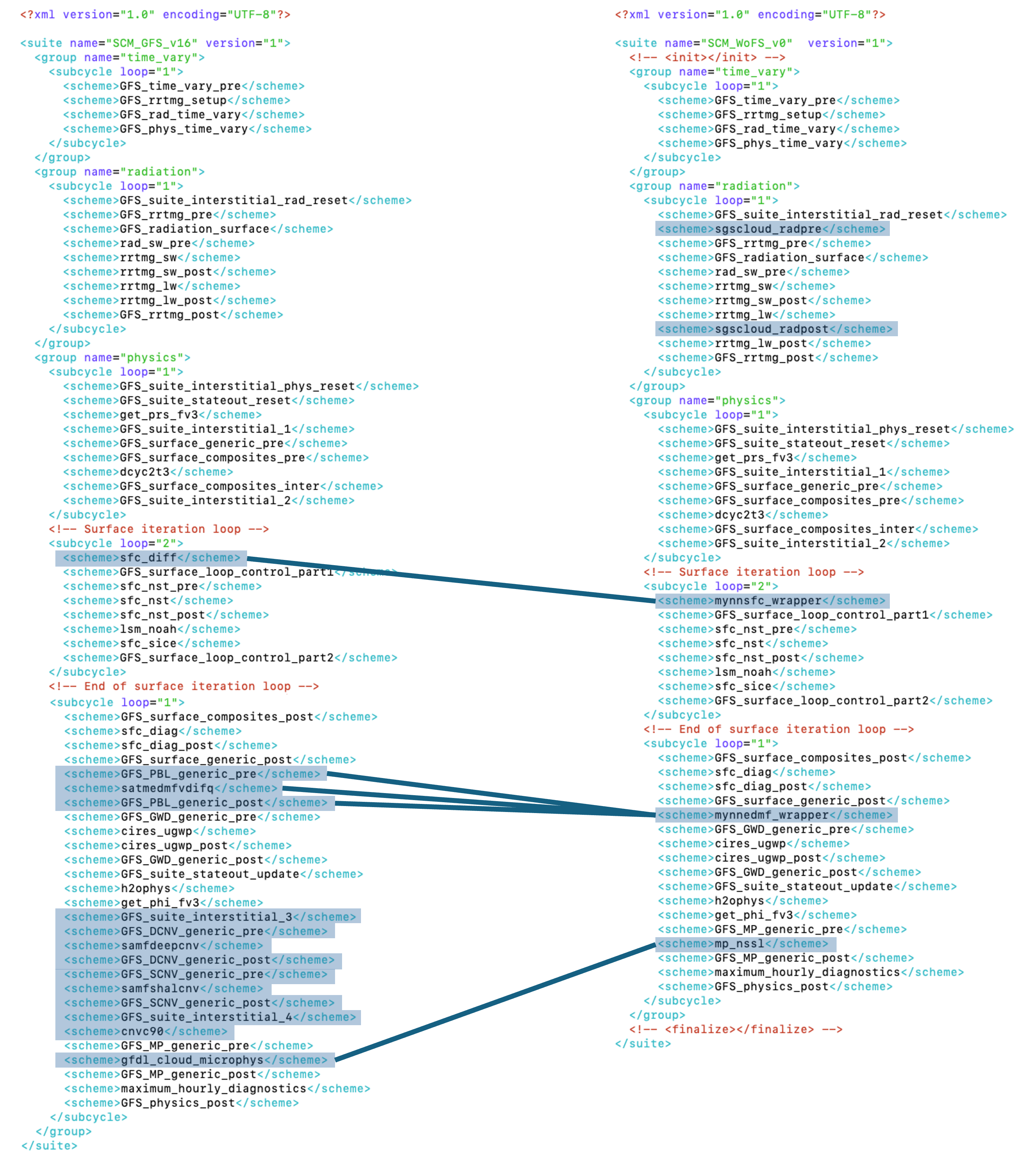
Q: What are some parameterizations used in suite WoFS_v0 that are not used in suite GFS_v16?
A: Coupling of subgridscale cloudiness and RRTMG radiation scheme (sgscloud_radpre and sgscloud_radpost), the Mellow-Yamada-Nakanishi-Niino (MYNN) surface layer (mynnsfc_wrapper) and planetary boundary layer (mynnedmf_wrapper) schemes. Also note that the GFS_v16 invokes a deep convective parameterization (samfdeepcnv), while suite WoFS_v0 does not. For this reason, suite WoFS_v0 is best suited for convective-allowing models.
Review the case configuration namelists and case input data file
Now navigate to the directory where case setup namelists are stored to see what you are going to run.
ls
Look at twpice.nml to see what kinds of information are required to set up an experiment.
Each case also has a NetCDF file in DEPHY format associated with it (determined by the case_name variable) that contains the initial conditions and forcing data for the case. Take a look at one of the files to see what kind of information is expected:
There are scalar variables (single values relevant for the simulation), initial condition variables (function of vertical level only), and forcing variables (function of time and/or vertical level). Note that not all forcing variables are required to be non-zero. Additionally, there are global attributes which define the forcing type for the case.
Run the SCM
Now that you have an idea of what the physics suites contain and how to set up cases, you can run the SCM.
The following commands will get you in the bin directory and run the SCM for the TWP-ICE case using all six supported suites.
Note: if you are using a Docker container, add -d at the end of the following command
Upon a successful run, the screen output should say that the runs completed successfully and the following subdirectories will be created in $SCM_WORK/ccpp-scm/scm/run/, each of them with a log file and results in NetCDF format in file output.nc:
output_twpice_SCM_GFS_v16, output_twpice_SCM_GFS_v16_RRTMGP, output_twpice_SCM_GFS_v17_p8_ugwpv1, output_twpice_SCM_HRRR_gf, and output_twpice_SCM_WoFS_v0
Any standard NetCDF file viewing or analysis tools may be used to examine the output file (ncdump, ncview, Python, etc).
Analyze the SCM results
The output directory for each case is controlled by its case configuration namelist. For this exercise, a directory containing the output for each integration is placed in the $SCM_WORK/ccpp-scm/scm/run/ directory. Inspect that the output directories now contain a populated output.nc file.
At this point, you use whatever plotting tools you wish to examine the output. For this course, we will use the basic Python scripts that are included in the repository. The main script is called scm_analysis.py and expects a configuration file as an argument. The configuration file specifies which output files to read, which variables to plot, and how to do so.
Set up the python environment needed to run the analysis script. First create the environment using a YAML file (only once) and activate the environment using conda.
conda env create -f environment-scm_analysis.yml
conda activate env_scm_analysis
Change into the following directory:
Copy Python plotting module needed for tutorial:
Run the following to generate plots for the TWP-ICE case:
Note: if you are using a Docker container, add -d at the end of the following command
You will notice some harmless messages pertaining to “Missing variables”, which are just meant to alert the user that some suites do not have certain types of parameterizations. Therefore, tendencies for those types of parameterizations are set to zero.
The script creates a new subdirectory within the
$SCM_WORK/ccpp-scm/scm/run/ directory called plots_twpice_all_suites
Change into that directory using the command
For docker, this directory is /home/plots_twpice_all_suites/comp/active. This is also mounted outside of the container, so you can exit the container and view the output files on your home file system in the directory $OUT_DIR/plots_twpice_all_suites/comp/active.
This directory contains various plot files in PDF format. Open the files and inspect the various plots such as the precipitation time series and the mean profiles of water vapor specific humidity, cloud water mixing ratio, temperature, and temperature tendencies due to forcing and physics processes.
Q: Examine the prediction of precipitation in file time_series_tprcp_rate_accum.pdf. Would you say that the rain rate is well predicted in the SCM simulations?
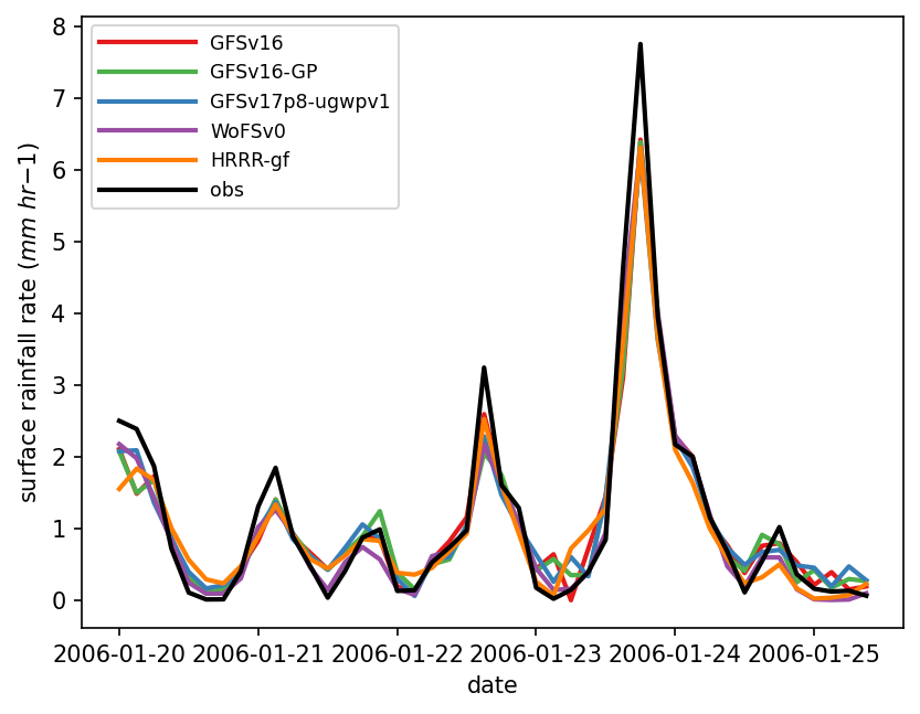
A: All supported suites reasonably predict the evolution of rain rate as a function of time and the results for all suites are similar, indicating that, for this variable, the commonality of forcing is a stronger factor in determining the results than the differences among suites. However, it should be noted that none of the suites capture the magnitude of the largest four precipitation events.
Q: Examine the profiles of temperature bias in file profiles_bias_T.pdf. In the lower troposphere (between the surface and 600 hPa), which suite(s) have a positive bias and which have a negative bias? In absolute terms, which suite has the highest bias in the lower troposphere?
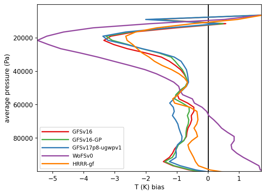
A: In the lower atmosphere, suite WoFS_v0 have a positive bias (that is, it is too warm compared to observations), while all other suites have a negative bias (that is, are too cold compared to observations). In the middle atmosphere, all suites have a negative temperature bias. Suite WoFS_v0 has the largest absolute bias, which reaches -5 K.
Q: Look at the tendencies due to deep and shallow convection in file profiles_mean_multi_conv_tendencies.pdf. Considering all suites, at approximately which level do the deep convective tendencies peak? And the shallow convection tendencies? Why are the convective tendencies for suite WoFS_v0 zero?
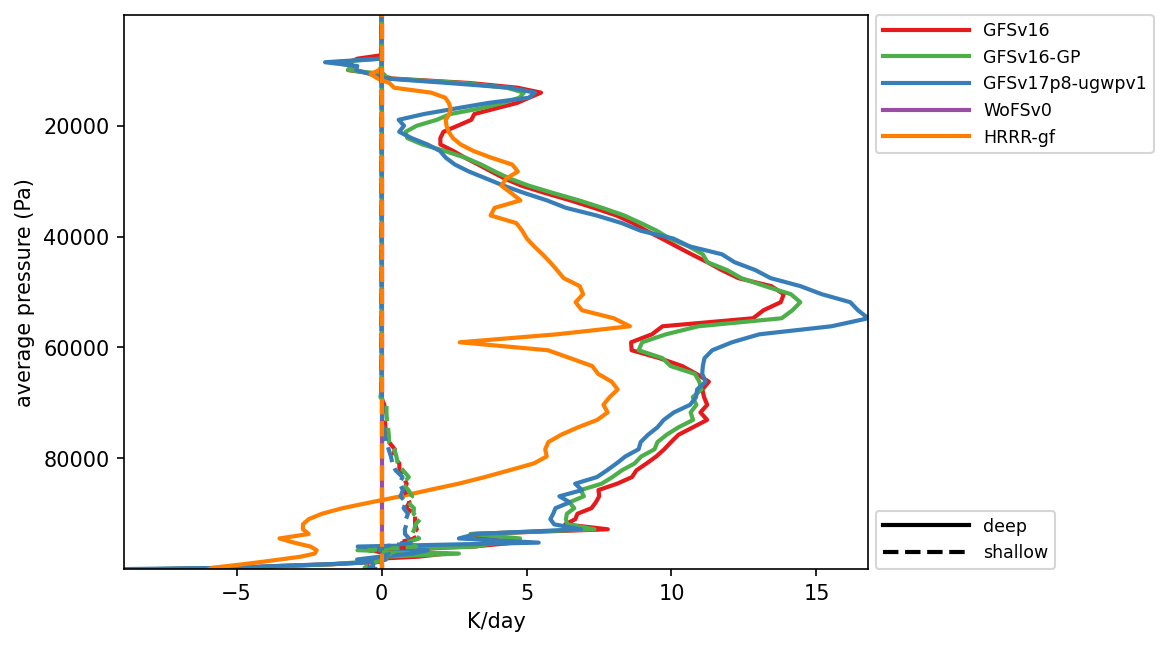
A: The deep convective scheme represents cumulus clouds that span the entire troposphere and their tendencies peak at approximately 500 hPa. The shallow convective scheme represents clouds at the top of the planetary boundary layer, with maximum tendencies at approximately 950 hPa .Suite WoFs_v0 does not produce any convective tendencies since it does not include a convective scheme because it is targeted for convective-allowing resolutions.
Q: Since it does not include a convective parameterization, is it appropriate to use suite WoFS_v0 for the SCM TWP-ICE case?
A: No, suite WoFS_v0 is included with the SCM as-is for research purposes but it is not expected to produce reasonable results for the TWP-ICE case or other CCPP SCM cases involving deep convection. This is because forcing for existing cases assumes a horizontal scale for which deep convection is subgrid-scale and is expected to be parameterized. The WoFS_v0 suite was designed for use in simulations with horizontal scale small enough not to need a deep convection parameterization active, and it does not contain a deep convective scheme. For suite WoFS_v0 to produce reasonable results with the SCM, the forcing would have to be modified to account for deep convection.
Exercise 2: Create a new CCPP suite
Exercise 2: Create a new CCPP suite
Create a new CCPP suite, re-run the SCM, and inspect the output
In this exercise you will learn how to create a new suite and use it with the SCM. A new suite can have many different levels of sophistication. Here we will explore the simplest case, which is to add an existing CCPP physics scheme to an existing suite. In particular, we will create a modified version of the WoFS_v0 suite that contains a convective parameterization, in this case the Simplified Arakawa Schubert (SAS) scheme. One might find it useful to employ a convective parameterization (CP) when the model grid is too coarse to explicitly allow convection and when using a SCM with a forcing dataset that represents an average over a large area (such as the datasets distributed with CCPP v7.0.0).
Note that no effort has been made to optimize the inter-parameterization communication in this new suite (for example, how microphysics and convection exchange information). This new suite is offered as a technical exercise only and its results should be interpreted with caution. If you want to learn more about creating suites, read the chapter on constructing suites in the CCPP Technical Documentation as it describes how Suite Definition Files (SDFs) are constructed.
This exercise has four steps:
- Create a New Suite Definition File for Suite SCM_WoFS_v0_sas
- Prepare the Namelist File for the New Suite
- Rebuild the SCM
- Run the SCM and Inspect the Output
Step 1: Create a New Suite Definition File for suite SCM_WoFS_v0_sas
You will create a new SDF based on the SCM_WoFS_v0, but with the scale-aware SAS cumulus scheme. Note that interstitial schemes must also be added.
cp suite_SCM_WoFS_v0.xml suite_SCM_WoFS_v0_sas.xml
Edit ccpp/suites/suite_SCM_WoFS_v0_sas.xml and
- Change the suite name to “SCM_WoFS_v0_sas”
- Add the scale-aware SAS deep and shallow cumulus schemes, the associated scheme/generic interstitial schemes, and the convective cloud cover diagnostic scheme to the “physics” group. The schemes you need to add are listed in bold below. You can also copy the new SDF instead of creating your own.
- Please note that the order of schemes within groups of a suite definition file is the order in which they will be executed. In this case, the placement of the schemes follows the placement of convective schemes from other GFS-based suites. In particular, deep convection precedes shallow convection and both need to appear in the time-split section of the “slow physics” part of the suite and before the microphysics scheme is called. Decisions about the order of schemes in general are guided by many factors related to physics-dynamics coupling, including numerical stability, and should be considered carefully. For example, one of the considerations should be to understand the “data flow” within a suite for each variable used within the added schemes, e.g. when/where the variables are modified in pre-existing schemes. This can be achieved by examining the variables’ Fortran “intents” in the pre-existing schemes’ metadata.
The suite name SCM_WoFS_v0_sas is listed below with the necessary additions highlighted in bold.
<suite name="SCM_WoFS_v0_sas" version="1">
<!-- <init></init> -->
<group name="time_vary">
<subcycle loop="1">
<scheme>GFS_time_vary_pre</scheme>
<scheme>GFS_rrtmg_setup</scheme>
<scheme>GFS_rad_time_vary</scheme>
<scheme>GFS_phys_time_vary</scheme>
</subcycle>
</group>
<group name="radiation">
<subcycle loop="1">
<scheme>GFS_suite_interstitial_rad_reset</scheme>
<scheme>sgscloud_radpre</scheme>
<scheme>GFS_rrtmg_pre</scheme>
<scheme>GFS_radiation_surface</scheme>
<scheme>rad_sw_pre</scheme>
<scheme>rrtmg_sw</scheme>
<scheme>rrtmg_sw_post</scheme>
<scheme>rrtmg_lw</scheme>
<scheme>sgscloud_radpost</scheme>
<scheme>rrtmg_lw_post</scheme>
<scheme>GFS_rrtmg_post</scheme>
</subcycle>
</group>
<group name="physics">
<subcycle loop="1">
<scheme>GFS_suite_interstitial_phys_reset</scheme>
<scheme>GFS_suite_stateout_reset</scheme>
<scheme>get_prs_fv3</scheme>
<scheme>GFS_suite_interstitial_1</scheme>
<scheme>GFS_surface_generic_pre</scheme>
<scheme>GFS_surface_composites_pre</scheme>
<scheme>dcyc2t3</scheme>
<scheme>GFS_surface_composites_inter</scheme>
<scheme>GFS_suite_interstitial_2</scheme>
</subcycle>
<!-- Surface iteration loop -->
<subcycle loop="2">
<scheme>mynnsfc_wrapper</scheme>
<scheme>GFS_surface_loop_control_part1</scheme>
<scheme>sfc_nst_pre</scheme>
<scheme>sfc_nst</scheme>
<scheme>sfc_nst_post</scheme>
<scheme>lsm_noah</scheme>
<scheme>sfc_sice</scheme>
<scheme>GFS_surface_loop_control_part2</scheme>
</subcycle>
<!-- End of surface iteration loop -->
<subcycle loop="1">
<scheme>GFS_surface_composites_post</scheme>
<scheme>sfc_diag</scheme>
<scheme>sfc_diag_post</scheme>
<scheme>GFS_surface_generic_post</scheme>
<scheme>mynnedmf_wrapper</scheme>
<scheme>GFS_GWD_generic_pre</scheme>
<scheme>cires_ugwp</scheme>
<scheme>cires_ugwp_post</scheme>
<scheme>GFS_GWD_generic_post</scheme>
<scheme>GFS_suite_stateout_update</scheme>
<scheme>h2ophys</scheme>
<scheme>get_phi_fv3</scheme>
<scheme>GFS_DCNV_generic_pre</scheme>
<scheme>samfdeepcnv</scheme>
<scheme>GFS_DCNV_generic_post</scheme>
<scheme>GFS_SCNV_generic_pre</scheme>
<scheme>samfshalcnv</scheme>
<scheme>GFS_SCNV_generic_post</scheme>
<scheme>cnvc90</scheme>
<scheme>GFS_MP_generic_pre</scheme>
<scheme>mp_nssl</scheme>
<scheme>GFS_MP_generic_post</scheme>
<scheme>maximum_hourly_diagnostics</scheme>
<scheme>GFS_physics_post</scheme>
</subcycle>
</group>
<!-- <finalize></finalize> -->
</suite>
Note: If you don’t want to type, you can copy a pre-generated SDF into place:
The detailed explanation of each primary physics scheme can be found in the CCPP Scientific Documentation. A short explanation of each scheme is below:
Step 2: Prepare the Namelist File for the New Suite
We will use the default WoFS_v0 namelist input file to create the namelist file for the new suite:
cp input_WoFS_v0.nml input_WoFS_v0_sas.nml
Next, edit file input_WoFS_v0_sas.nml and modify the following namelist options to conform with the deep/shallow saSAS cumulus schemes in the SDF file :
shal_cnv = .true.
do_deep = .true.
imfdeepcnv = 2
imfshalcnv = 2
Check the Description of Physics Namelist Options for information.
Note: If you don’t want to type, you can copy a pre-generated namelist into place:
Step 3: Rebuild the SCM
Now follow these commands to rebuild the SCM with the new suite included:
cmake ../src -DCCPP_SUITES=ALL
make -j4
In addition to defining a SDF for a new suite, which only contains information about which schemes are used, one also needs to define parameters needed by the schemes in the suite (namelist file) as well as which tracers (tracer file) the SCM should carry that a given physics suite expects. There are two ways to provide this information at runtime.
- The first way is by giving command line arguments to the run script. For the namelist file, specify it with -n namelist_file.nml (assuming that the namelist file is in $SCM_WORK/ccpp-scm/ccpp/physics_namelists). For the tracer file, specify it with -t tracer_file.txt (assuming the tracer file is in $SCM_WORK/ccpp-scm/scm/etc/tracer_config).
- The second way is to define default namelist and tracer configuration files associated with the new suite in the $SCM_WORK/ccpp-scm/scm/src/suite_info.py file, where a Python list is created containing default information for the SDFs.
If you are planning on using a new suite more than just for testing purposes, it makes sense to use the second method so that you don’t have to continually use the -n and -t command line arguments when using the new suite to run the SCM.
If you try to run the SCM using a new suite and don’t specify a namelist and a tracer configuration file using either method, the run script will generate a fatal error.
For the purpose of this tutorial, you will add new default values for the new suite to make your life easier, option 2. Edit $SCM_WORK/ccpp-scm/scm/src/suite_info.py to add default namelist and tracer files associated with two suites that we will create in this tutorial (the second suite has yet to be discussed, but let’s add it now for expediency):
suite_list.append(suite('SCM_GFS_v16', 'tracers_GFS_v16.txt', 'input_GFS_v16.nml', 600.0, 1800.0, True ))
suite_list.append(suite('SCM_GFS_v17_p8', 'tracers_GFS_v17_p8.txt', 'input_GFS_v17_p8.nml', 600.0, 600.0, True ))
suite_list.append(suite('SCM_RAP', 'tracers_RAP.txt', 'input_RAP.nml', 600.0, 600.0 , True ))
suite_list.append(suite('SCM_RRFS_v1beta', 'tracers_RRFS_v1beta.txt', 'input_RRFS_v1beta.nml', 600.0, 600.0 , True ))
suite_list.append(suite('SCM_WoFS_v0', 'tracers_WoFS_v0.txt', 'input_WoFS_v0.nml', 600.0, 600.0 , True ))
suite_list.append(suite('SCM_HRRR', 'tracers_HRRR.txt', 'input_HRRR.nml', 600.0, 600.0 , True ))
suite_list.append(suite('SCM_WoFS_v0_sas', 'tracers_WoFS_v0.txt', 'input_WoFS_v0_sas.nml', 600.0, 600.0 , False))
suite_list.append(suite('SCM_WoFS_v0_sas_sfcmod', 'tracers_WoFS_v0.txt', 'input_WoFS_v0_sas.nml', 600.0, 600.0 , False))
Note: If you don’t want to type, you can copy pre-generated files into place:
Step 4: Run the Model and Inspect Output
Execute the following command to run the SCM for the TWP-ICE case using the new suite. Note that you don’t need to specify a tracer or namelist file since default ones now exist for this new suite.
Note: if you are using a Docker container, add -d at the end of the command
Upon completion of build, the following subdirectory will be created with a log file and results in NetCDF format in file output.nc:
$SCM_WORK/ccpp-scm/scm/run/output_twpice_SCM_WoFS_v0_sas
In order to generate graphics, first prepare a configuration file for the plotting script using the commands below.
Change into the following directory:
cp plot_configs/twpice_all_suites.ini plot_configs/twpice_scm_tutorial.ini
Edit plot_configs/twpice_scm_tutorial.ini. Since we only want to check how the scale-aware SAS scheme impacts the default WoFS_v0 suite, simply list the two suites in the first two lines of the file. Note that the second line defines the labels of the lines in the output plots and the third line defines the output directory for the plots.
scm_datasets_labels = WoFSv0, WoFSv0_sas
plot_dir = plots_twpice_WoFSv0_sas/
Note: If you don’t want to type, you can copy over a pre-generated plot configuration file:
Change into the following directory:
ln -s $SCM_WORK/ccpp-scm/scm/etc/scripts/plot_configs/twpice_scm_tutorial.ini twpice_scm_tutorial.ini
Create the plots with the new suite with the command below.
Note: if you are using a Docker container, add -d at the end of the command
The script creates a new subdirectory within the $SCM_WORK/ccpp-scm/scm/run/ directory called plots_twpice_WoFSv0_sas/comp/active and places the graphics in there. Open the files and inspect the various plots for changes introduced by adding a convective parameterization.
Inspect the SCM Results
Q: Examine the prediction of precipitation in file time_series_tprcp_rate_accum.pdf. How does the new suite change the precipitation?
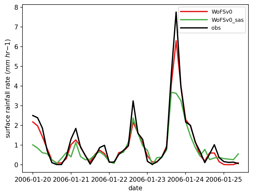
A: The time series of precipitation shows that WoFS_v0 with or without saSAS deep and shallow schemes produces similar results.
Q: Examine the profiles of temperature bias in file profiles_bias_T.pdf. How does adding a convective parameterization affect the vertical distribution of temperature bias?
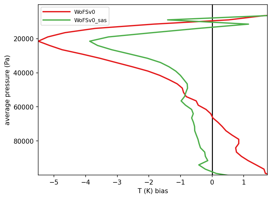
A: It is interesting to see that, when a cumulus scheme is added, the positive temperature bias below 600 hPa is adjusted to -1 K and the negative bias around the 200 hPa is adjusted to -3.5 K, which is similar to the bias of other physics suites designed for applications in coarser grid spacing, as seen in the previous exercise.
Exercise 3: Add a new CCPP-compliant scheme
Exercise 3: Add a new CCPP-compliant scheme
Adding a New CCPP-Compliant Scheme
In this exercise you will learn how to implement a new scheme in CCPP. This will be a simple case in which all variables that need to be passed to and from the physics are already defined in the host model and available for the physics. You will create a new CCPP-compliant scheme to modify the sensible and latent heat fluxes by adding a tunable amount to each of them. You will then implement the new scheme, which we will call fix_sys_bias_sfc, in the SCM_WoFS_v0 suite. Note that this procedure is provided only as an exercise to examine the impact of the surface fluxes on the prediction. While correcting the surface fluxes can help fix systematic biases, there is no scientific basis for arbitrarily modifying the fluxes in this case.
This exercise has four steps:
- Prepare a CCPP-compliant scheme
- Add the scheme to the Cmake list of files
- Add the scheme to the Suite Definition File
- Run the model and inspect the output
Step 1: Prepare a CCPP-compliant Scheme
The first step is to prepare a new CCPP-compliant scheme, which in this case will be called fix_sys_bias_sfc and will be responsible for “tuning” the surface fluxes. A skeleton CCPP-compliant scheme is provided for you to download into your codebase and continue developing. Two skeleton files fix_sys_bias_sfc.F90 and fix_sys_bias_sfc.meta, which are the scheme itself and the metadata file with the description of the variables passed to and from the scheme, respectively, need to be copied from tutorial_files/ directory and into the CCPP physics source code directory:
cp $SCM_WORK/tutorial_files/add_new_scheme/fix_sys_bias_sfc_skeleton.meta $SCM_WORK/ccpp-scm/ccpp/physics/physics/SFC_Layer/MYNN/fix_sys_bias_sfc.meta
In the file fix_sys_bias_sfc.F90, you will need to add the following modifications to the subroutine fix_sys_bias_sfc_run:
- Add hflx_r and qflx_r which correspond to the sensible and latent heat flux, respectively, to the argument list in subroutine fix_sys_bias_sfc_run with
subroutine fix_sys_bias_sfc_run (im, con_cp, con_rd, con_hvap, p1, t1, hflx_r, qflx_r, errmsg, errflg)
- Declare and allocate variables hflx_r and qflx_r
real(kind=kind_phys), intent(inout) :: hflx_r(:), qflx_r(:)
...
- Add code to modify the surface fluxes by adding a tunable amount of each of them or, in case of negative fluxes, setting the fluxes to zero. Note that the modification factors are converted to kinematic units since the variables hflx_r and qflx_r are in kinematic units, not W m2.
rho = p1(i)/(con_rd*t1(i))
!convert mod_factor to kinematic units and add
hflx_r(i) = MAX(sens_mod_factor/(rho*con_cp) + hflx_r(i), 0.0)
qflx_r(i) = MAX(lat_mod_factor/(rho*con_hvap) + qflx_r(i), 0.0)
end do
Where con_rd (287.05 J kg-1 K-1; ideal gas constant for dry air), con_cp (1004.6 J kg-1 K-1; specific heat of dry air at constant pressure), and con_hvap (2.5106 J kg-1; latent heat of evaporation and sublimation) are constants defined in the host model ($SCM_WORK/ccpp-scm/scm/src/scm_physical_constants.F90), and sens_mod_factor and lat_mod_factor are arbitrary constants defined locally:
real(kind=kind_phys), parameter :: lat_mod_factor = 40 !W m-2
Given the value of the constants, this results in an increase of 40 W m-2 to the surface latent heat flux, while the sensible heat flux is not altered.
After saving your changes, edit the corresponding metadata file: fix_sys_bias_sfc.meta to add variables hflx_r and qflx_r after the entry for variable t1. The order of the variables on the table should match the order of the arguments in the subroutine call.
The metadata file needs to be populated with the same variables as the subroutine fix_sys_bias_sfc_run call:
standard_name = air_temperature_at_surface_adjacent_layer
long_name = mean temperature at lowest model layer
units = K
dimensions = (horizontal_loop_extent)
type = real
kind = kind_phys
intent = in
[qflx_r]
standard_name = surface_upward_specific_humidity_flux
long_name = kinematic surface upward latent heat flux
units = kg kg-1 m s-1
dimensions = (horizontal_loop_extent)
type = real
kind = kind_phys
intent = inout
[hflx_r]
standard_name = surface_upward_temperature_flux
long_name = kinematic surface upward sensible heat flux
units = K m s-1
dimensions = (horizontal_loop_extent)
type = real
kind = kind_phys
intent = inout
[errmsg]
…
Note: If you don’t want to type, you can copy over completed versions of these files:
cp $SCM_WORK/tutorial_files/add_new_scheme/fix_sys_bias_sfc.meta $SCM_WORK/ccpp-scm/ccpp/physics/physics/SFC_Layer/MYNN
Step 2: Add the Scheme To the Cmake List of Files
Now that the CCPP-compliant scheme fix_sys_bias_sfc.F90 and the accompanying fix_sys_bias_sfc.meta are complete, it is the time to add the scheme to the CCPP prebuild configuration.
Edit file $SCM_WORK/ccpp-scm/ccpp/config/ccpp_prebuild_config.py and include scheme fix_sys_bias_sfc.F90 in the SCHEME_FILES section:
...
'ccpp/physics/physics/SFC_Layer/MYNN/mynnsfc_wrapper.F90' ,
'ccpp/physics/physics/SFC_Layer/MYNN/fix_sys_bias_sfc.F90' ,
...
Note: If you don’t want to type, you can copy over completed version:
Step 3: Add the Scheme To the Suite Definition File
The next step is to create a new Suite Definition File (SDF) and edit it so that it lists the scheme fix_sys_bias_sfc just after the GFS_surface_generic_post interstitial scheme:
First, create a new SDF from an existing SDF.
cp suite_SCM_WoFS_v0_sas.xml suite_SCM_WoFS_v0_sas_sfcmod.xml
Next, the new SDF, suite_SCM_WoFS_v0_sas_sfcmod.xml, needs the following modifications:
- Change the suite name to “SCM_WoFS_v0_sas_sfcmod”
- Add the scheme “fix_sys_bias_sfc” after GFS_surface_generic_post
Note: If you don’t want to type, you can copy the completed SDF and modified supported suite_list:
cp $SCM_WORK/tutorial_files/create_new_suite/suite_info.py $SCM_WORK/ccpp-scm/scm/src/suite_info.py
Step 4: Run the Model and Inspect the Output
After creating the new SDF, follow these commands to rebuild the SCM executable:
cmake ../src -DCCPP_SUITES=ALL
make -j4
The following two commands will run the SCM for the TWP-ICE case using the modified suite containing the fix_sys_bias_sfc scheme, respectively.
Note: if you are using a Docker container, add -d at the end of the command
Upon completion of the run, the following subdirectory will be created containing a log file and results in NetCDF format in file output.nc:
$SCM_WORK/ccpp-scm/scm/run/output_twpice_SCM_WoFS_v0_sas_sfcmod
Now you will create plots to visualize the results. Edit $SCM_WORK/ccpp-scm/scm/etc/scripts/plot_configs/twpice_scm_tutorial.ini to define the results that will be displayed: the WoFS_v0_sas results (which use the saSAS scheme), and the new results obtained with the surface fluxes modification:
output_twpice_SCM_WoFS_v0_sas_sfcmod/output.nc
scm_datasets_labels = WoFSv0_sas,WoFSv0_sas_sfcmod
plot_dir = plots_twpice_sas_sfcmod/
Note: If you don’t want to type, you can copy over a pre-generated plot configuration file:
Change into the following directory:
Create the plots for the new suite with the command below.
Note: if you are using a Docker container, add -d at the end of the command
The new plots are under:
$SCM_WORK/ccpp-scm/scm/run/plots_twpice_sas_sfcmod/comp/active/
Inspect the SCM results
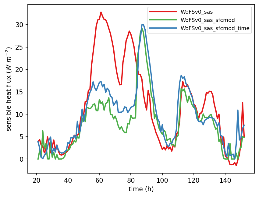
Q: Examine the time series of latent and sensible heat fluxes in files time_series_lhf.pdf and time_series_shf.pdf, respectively. Are the modified latent and sensible heat fluxes as expected?
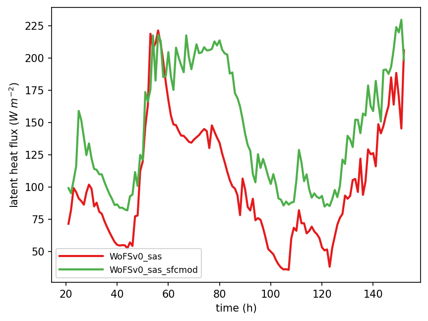
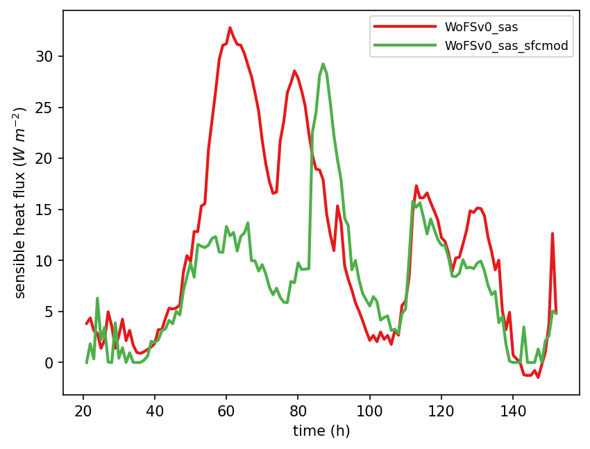
A: Compared to WoFSv0_sas, the surface latent heat flux in WoFSv0_sas_sfcmod is increased as expected, and the surface sensible heat flux adjusts to a lower value for much of the simulation.
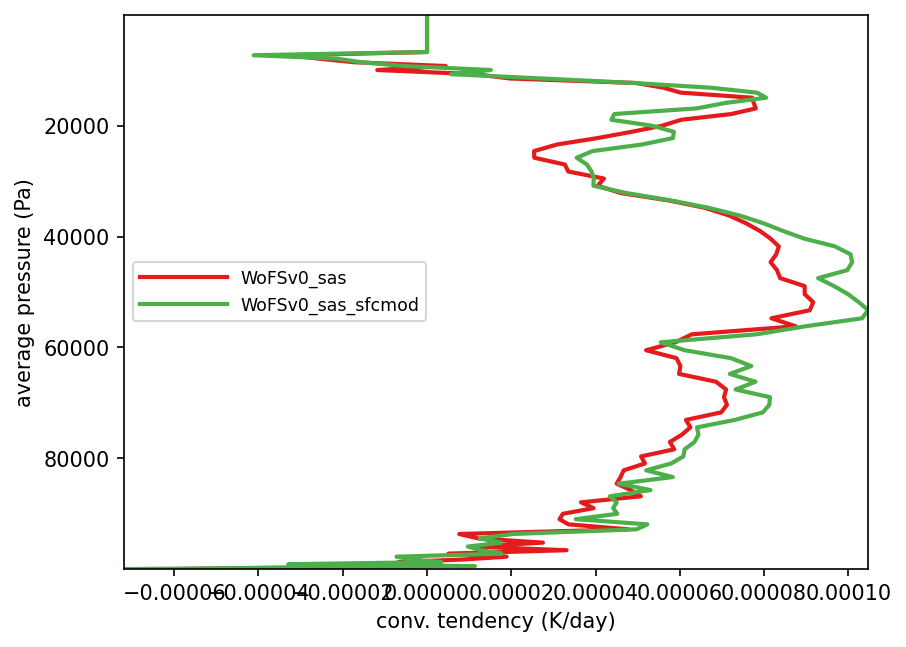
Q: Examine the vertical profile of convective tendencies in file profiles_mean_dT_dt_conv.pdf. How does the increased latent heat flux affect the atmospheric convection?
The evaporation process associated with the increased surface latent heat flux makes more moisture available in the atmosphere, which triggers stronger convection.
A: This exercise shows us that if some properties of the surface energy budget system change in such a way that the surface latent heat flux goes up, the system will rebalance to compensate for this change. In this case, we note that the sensible heat flux was reduced for much of the forecast, even though we did not modify it directly. The sensible heat flux depends on the difference in temperature between the sea surface temperature and the air, the wind speed, and the surface heat exchange coefficient. Given that sea surface temperature changes very slowly, the changes in sensible heat flux can be attributed to lowering of the air temperature or increase in the wind speed. Those are non-linear effects deriving from the increase in latent heat flux.
Exercise 4: Add a new variable
Exercise 4: Add a new variable
Add a new variable to a CCPP-compliant scheme
Adding a New Variable
In this section, we will explore how to pass a new variable onto an existing scheme. The surface latent and sensible heat fluxes will be adjusted in scheme fix_sys_bias_sfc to be time-dependent using the existing variable solhr (time in hours after 00 UTC at the current timestep). The surface fluxes will now only be modified between the hours of 20:30 and 8:30 UTC, which correspond to the hours of 6:00 AM and 6:00 PM local time in Darwin, Australia, where this case is located.
Step 1: Add Time Dependency to the fix_sys_bias_sfc_time Scheme
Edit file $SCM_WORK/ccpp-scm/ccpp/physics/physics/fix_sys_bias_sfc.F90 and add solhr to the argument list for subroutine fix_sys_bias_sfc_run:
Then declare solhr as a real variable:
Next, add the time-dependent surface flux modification using an if statement between the CCPP error message handling and the do loop:
A metadata entry should be added to the table for subroutine fix_sys_bias_sfc_run in file $SCM_WORK/ccpp-scm/ccpp/physics/physics/fix_sys_bias_sfc.meta.
standard_name = air_temperature_at_surface_adjacent_layer
long_name = mean temperature at lowest model layer
units = K
dimensions = (horizontal_loop_extent)
type = real
kind = kind_phys
intent = in
[solhr]
standard_name = forecast_utc_hour
long_name = time in hours after 00z at the current timestep
units = h
dimensions = ()
type = real
kind = kind_phys
intent = in
[hflx_r]
...
Note: If you don’t want to type, you can copy over completed versions of these files:
cp $SCM_WORK/tutorial_files/add_new_variable/fix_sys_bias_sfc.meta $SCM_WORK/ccpp-scm/ccpp/physics/physics/SFC_Layer/MYNN
Since solhr is an existing variable, you do not need to modify the host model. Additionally, no changes are needed in the SDF or in the prebuild script since you are simply modifying a scheme and not adding a new scheme. You can proceed to rebuilding the SCM.
Step 2: Build the Executable, Run the Model, and Inspect the Output
Issue these commands to rebuild the SCM executable:
cmake ../src -DCCPP_SUITES=ALL
make -j4
In order to avoid overwriting the output produced in exercise “Add a new scheme”, first rename the output directory:
The following command will run the SCM for the TWP-ICE case using suite WoFS_v0_sas_sfcmod with scheme fix_sys_bias_sfc modified to use variable solhr:
Note: if you are using a Docker container, add -d at the end of the command
Upon completion of the run, the following subdirectory will be created, with a log file and results in NetCDF format in file output.nc:
$SCM_WORK/ccpp-scm/scm/run/output_twpice_SCM_WoFS_v0_sas_sfcmod
To visualize the results, edit file $SCM_WORK/ccpp-scm/scm/etc/scripts/plot_configs/twpice_scm_tutorial.ini and add the new test directory name and label name to the first two lines:
output_twpice_WSAS_sfcmod/output.nc, output_twpice_SCM_WoFS_v0_sas_sfcmod/output.nc
scm_datasets_labels = WoFSv0_sas,WoFSv0_sas_sfcmod,WoFSv0_sas_sfcmod_time
plot_dir = plots_twpice_WoFSv0_sas_sfcmod_time/
Note: If you don’t want to type, you can copy over a pre-generated plot configuration file:
Change into the following directory:
Next, run the following command to generate plots for the last three exercises in this tutorial.
Note: if you are using a Docker container, add -d at the end of the command
The script creates a new subdirectory within the $SCM_WORK/ccpp-scm/scm/run/ directory called plots_twpice_R_sas_sfcmod_time/comp/active
Inspect the Results
Q: Examine the surface latent heat flux and the surface sensible heat flux in files time_series_lhf.pdf and time_series_shf.pdf, respectively. How does the latent heat flux differ from the previous exercise?
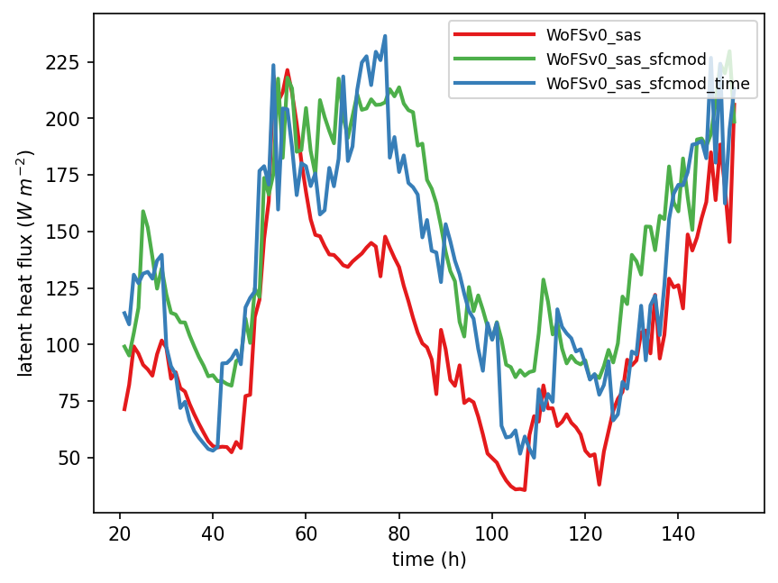
A: Instead of adding 40 W m-2 to the latent heat flux throughout the simulation, the latent heat flux value was modified only between the hours of 6 AM and 6 PM local time to mimic the observed diurnal cycle feature.
Q: Examine the temperature bias and the specific humidity bias in files profiles_bias_T.pdf and profiles_bias_qv.pdf, respectively. How are the temperature and moisture profiles affected by the surface latent heat flux modification?
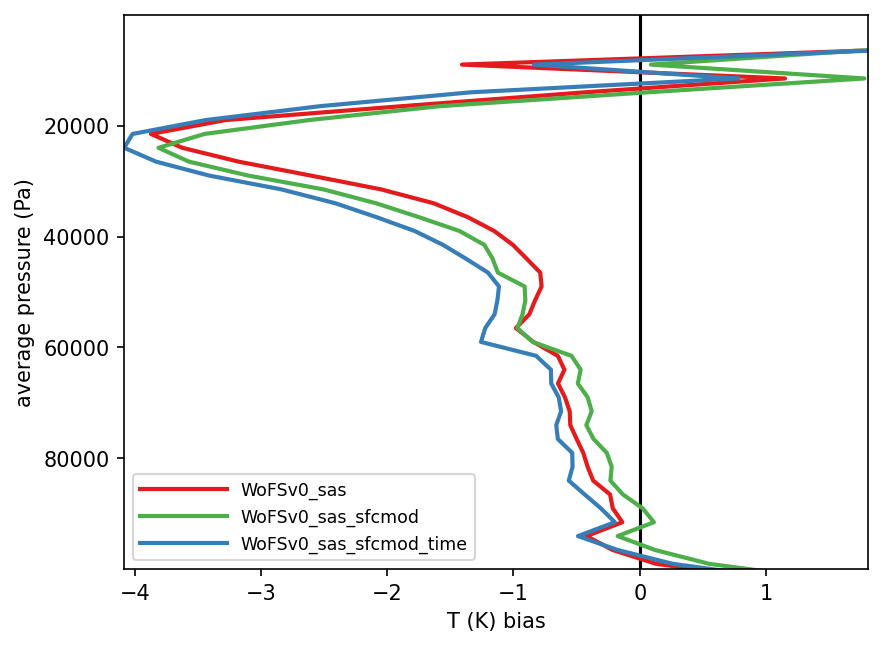

A: Even though we effectively added more energy to the atmosphere, the net effect in the T and q profiles are either neutral or show an increase in negative bias. This points out that physics suites have complicated non-linear interactions and that it is often possible to get unexpected results. This also points to the utility of studying physics in a SCM context, where one at least has a chance at understanding the mechanisms when only dealing with one column and are excluding interactions/feedbacks due the presence and advection from surrounding columns.
Contributing Development
Contributing Development
Contributing Development
The development process for the CCPP and SCM makes use of the tools git and GitHub for code development. There are three code repositories, and new development may be contributed to any or all of them.
The SCM and CCPP components are housed in authoritative (official) repositories. git submodules are used in the SCM to manage the CCPP subcomponents.
- All the authoritative repositories are read-only for users.
- Branches under the authoritative repositories include the main development (main) branch, production branches, and public release branches.
- Branches under the authoritative repositories are protected.
- New development will almost always start from the authoritative repository development branch, so that it can easily be merged.
First steps
1. Setup a GitHub Account. Go to https://github.com and create an account.
2. Create a GitHub issue in the repository where you will be doing development. This allows other developers to review your proposed work, make suggestions, and track progress as you work.
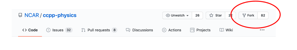
3. Create a fork via github:
- Login to your personal GitHub account
- Go to the official code repository website (e.g. https://github.com/NCAR/ccpp-physics)
- Click on “fork” on the top right corner. You will see the repository in your own GitHub account.
- A fork is a copy of an original repository on your GitHub account. You manage your own fork.
- Forks let you make changes to a project without affecting the original repository.
- You can fetch updates from the original repository.
- You can submit changes to the original repository with pull requests (PRs).
- For more details, please see Working with forks.
Clone the repository
Cloning a repository creates a copy on to your local machine. To begin a new development effort, you will need to start with the latest version of the repository development branch. For the CCPP and SCM repositories, this is the “main” branch. From this branch, you will create a new branch, and add your development there.
1. Clone the authoritative repository:
2. Update your remotes. Git uses a named remote to refer to repositories. By default, “origin” is the name for the repository from which this local copy was cloned. We will rename this to “upstream” and add a new remote for your own fork, for development.
git remote add origin https://github.com/<your_github_username>/ccpp-physics
3. Check out the main branch and create a new branch for your local development
git checkout -b feature/my_new_work
Expert Tip: Starting point for new development
New development will almost always start from the authoritative repository development branch, so that it can easily be merged. While you have been using a release tag for this tutorial, please use the latest code if you plan to contribute new development.
4. Push this branch to your fork as an initial starting point. First confirm your remotes
origin https://github.com/<your_github_username>/ccpp-physics (fetch)
origin https://github.com/<your_github_username>/ccpp-physics (push)
upstream https://github.com/NCAR/ccpp-physics (fetch)
upstream https://github.com/NCAR/ccpp-physics (push)
git push origin feature/my_new_work
Code Development
Now you are ready to begin development by modifying or adding files. Once you have some changes made, you should use your repository fork to archive them.
The git code development process uses frequent updates and detailed log messages to ensure that a detailed record of your changes can be reviewed by others. The basic steps are:
git commit --- to commit all of the changes that have been “added” by git add
git push --- to push these latest changes to your GitHub fork
More information about the git code development process can be found at: https://docs.github.com/en/github/using-git
Additional details describing the code development process for the UFS Weather Model, including how to handle nested submodules, can be found at: https://github.com/ufs-community/ufs-weather-model/wiki/Making-code-changes-in-the-UFS-weather-model-and-its-subcomponents
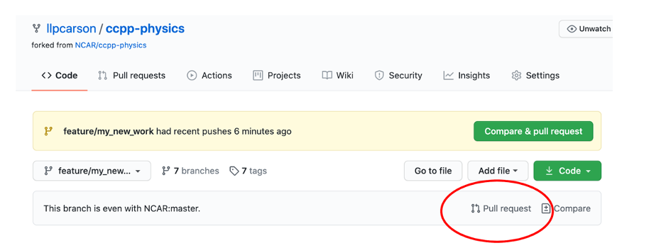
Pull Requests
A PR tells the code managers that your code changes from your feature branch are ready to undergo a review process for being merged into the main branch in the official repository.
Creating a PR
- Go to the your_github_account repository, choose your branch, then click on “Pull request”.
- In the next page, choose base repository and base branch. By default, PRs are based on the parent repository default branch, click “create pull request”.
- Provide a Title. If the PR is for production or release branch, put the production or release branch at the beginning of the title. E.g. “Release/public-v2: update build script.”
- Fill out the template
- Click on “Create Pull Request” or “Create Draft Pull Request” button.
Code review
- Reviews allow collaborators to comment on the changes proposed in pull requests, approve the changes, or request further changes before the pull request is merged.
- Anyone with read access can review and comment on the changes it proposes.
- Developers are expected to address the comments made by the reviewers.
- Reviewers are expected to review the code promptly so that the commit will not be delayed.
- Any code changes can be committed and pushed to your fork, and the PR will automatically update.
Code Commit
- After the code changes have been reviewed and approved by at least one code owner and any additional requested reviewers, the code owners will merge the changes into the main branch.
How to Get Help
How to Get Help
How to Get Help
User support is available for the CCPP SCM and CCPP. An overview of the CCPP User support can be found at: https://dtcenter.org/community-code/common-community-physics-package-ccpp/user-support
This site provides links to:
- Documentation
- FAQs
- Instructional Videos
- Online tutorials
- Developer Information
Send questions regarding any aspect of CCPP SCM or CCPP to GitHub Discussions at:
- https://github.com/NCAR/ccpp-physics/discussions
- https://github.com/NCAR/ccpp-framework/discussions
- https://github.com/NCAR/ccpp-scm/discussions
How to Provide Feedback on this Tutorial
Please consider taking a few minutes to complete our Tutorial survey, and thank you! Survey