Derecho Case (29 Jun 2012)
Derecho Case (29 Jun 2012)Case overview
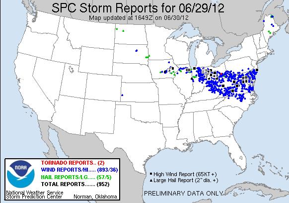
Reason for interest: Very strong, high-impact derecho
A deadly, record-setting derecho on this day was preceded by major instability from the Midwest to the East Coast of the United States, with CAPE values exceeding 5000 J/kg and temperatures reaching above 100°F (38°C). Elevated convection in northern Illinois moved into Indiana along a weak stationary front, above an elevated mixed layer. Record temperatures, abundant moisture, and steep lapse rates aided further storm development to the south and east. A squall line eventually formed into a bow echo and wreaked havoc from Illinois over the Appalachian Mountains all the way to the Atlantic coast.
More than 20 fatalities resulted from high winds and falling trees, and over 4 million people lost power. There were 893 high wind reports for June 29th, 2012, with some reaching over 90 mph.
SPC Storm Reports for June 29th, 2012:
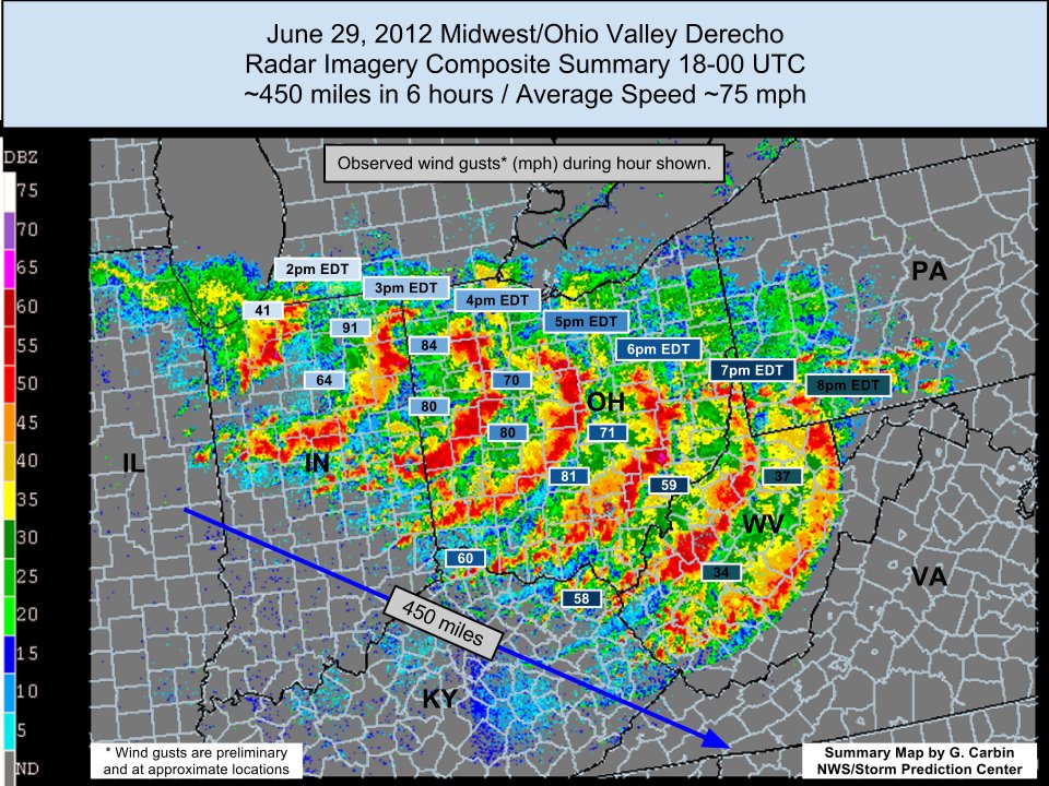
Storm Summary from NWS/SPC:
Set up environment
Set up environmentSet Up Environment
| tcsh | bash |
|---|---|
|
cd /home/ec2-user
setenv PROJ_DIR `pwd` setenv PROJ_VERSION 4.1.0
|
cd /home/ec2-user
export PROJ_DIR=`pwd` export PROJ_VERSION="4.1.0"
|
| For tcsh: | For bash: |
|---|---|
|
setenv CASE_DIR ${PROJ_DIR}/derecho
|
export CASE_DIR=${PROJ_DIR}/derecho
|
cd ${CASE_DIR}
mkdir -p wpsprd wrfprd gsiprd postprd pythonprd metprd metviewer/mysql
Extra step for singularity users
Users of singularity containerization software will need to set a special variable for temporary files written by singularity at runtime:
| tcsh | bash |
|---|---|
|
setenv TMPDIR ${PROJ_DIR}/derecho/tmp
|
export TMPDIR=${PROJ_DIR}/derecho/tmp
|
Run NWP initialization components
Run NWP initialization componentsRun NWP Initialization Components
The NWP workflow process begins by creating the initial and boundary conditions for running the WRF model. This will be done in two steps using WPS (geogrid.exe, ungrib.exe, metgrid.exe) and WRF (real.exe) programs.
Initialization Data
Global Forecast System (GFS) forecast files initialized at 12 UTC on 20120629 out 24 hours in 3-hr increments are provided for this case.
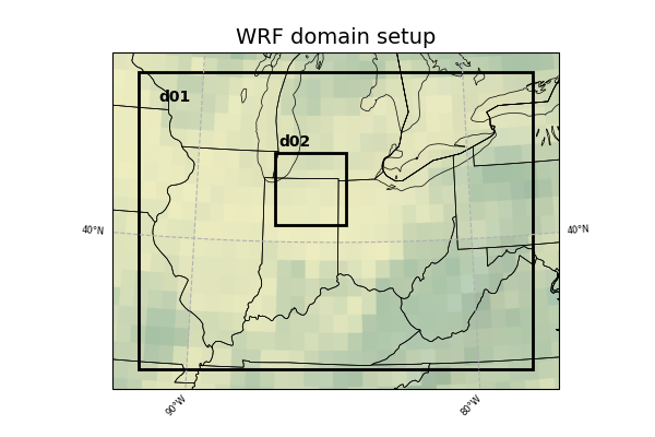
Model Domain
This case uses the nesting functionality of WRF: instead of one domain at a single resolution, this WRF run has one larger, coarser-resolution domain, and a smaller, finer-resolution domain within it. The outer WRF domain we have selected for this case covers the Ohio River region in the eastern United States, while the nested domain covers a portion of southern Ohio and far-northeastern Kentucky. The exact domains are shown below:
SELECT THE APPROPRIATE CONTAINER INSTRUCTIONS FOR YOUR SYSTEM BELOW:
Step One (Optional): Run Python to Create Image of Domain
A Python script has been provided to plot the computational domain that is being run for this case. If desired, run the dtcenter/python container to execute Python in docker-space using the namelist.wps in the local scripts directory, mapping the output into the local pythonprd directory.
-v ${PROJ_DIR}/container-dtc-nwp/components/scripts/common:/home/scripts/common \
-v ${PROJ_DIR}/container-dtc-nwp/components/scripts/derecho_20120629:/home/scripts/case \
-v ${PROJ_DIR}/data/shapefiles:/home/data/shapefiles \
-v ${CASE_DIR}/pythonprd:/home/pythonprd \
--name run-derecho-python dtcenter/python:${PROJ_VERSION} \
/home/scripts/common/run_python_domain.ksh
A successful completion of the Python plotting script will result in the following file in the pythonprd directory. This is the same image that is shown at the top of the page showing the model domain.
Step Two: Run WPS
Using the previously downloaded data (in ${PROJ_DIR}/data), while pointing to the namelists in the local scripts directory, run the dtcenter/wps_wrf container to run WPS in docker-space and map the output into the local wpsprd directory.
-v ${PROJ_DIR}/data/WPS_GEOG:/data/WPS_GEOG -v ${PROJ_DIR}/data:/data \
-v ${PROJ_DIR}/container-dtc-nwp/components/scripts/common:/home/scripts/common \
-v ${CASE_DIR}/wrfprd:/home/wrfprd -v ${CASE_DIR}/wpsprd:/home/wpsprd \
-v ${PROJ_DIR}/container-dtc-nwp/components/scripts/derecho_20120629:/home/scripts/case \
--name run-dtc-nwp-derecho dtcenter/wps_wrf:${PROJ_VERSION} /home/scripts/common/run_wps.ksh
Once WPS begins running, you can watch the log files being generated in another window by setting the ${CASE_DIR} environment variable and tailing the log files:
Type CTRL-C to exit the tail utility.
A successful completion of the WPS steps will result in the following files (in addition to other files) in the wpsprd directory
geo_em.d02.nc
FILE:2012-06-29_12
FILE:2012-06-29_15
FILE:2012-06-29_18
...
FILE:2012-06-30_09
FILE:2012-06-30_12
met_em.d01.2012-06-29_12:00:00.nc
met_em.d01.2012-06-29_15:00:00.nc
met_em.d01.2012-06-29_18:00:00.nc
...
met_em.d01.2012-06-30_09:00:00.nc
met_em.d01.2012-06-30_12:00:00.nc
met_em.d02.2012-06-30_03:00:00.nc
met_em.d02.2012-06-30_06:00:00.nc
met_em.d02.2012-06-30_09:00:00.nc
Step Three: Run real.exe
Using the previously downloaded data (in ${PROJ_DIR}/data), output from WPS in step one, and pointing to the namelists in the local scripts directory, run the dtcenter/wps_wrf container to this time run real.exe in docker-space and map the output into the local wrfprd directory.
-v ${PROJ_DIR}/data:/data -v ${PROJ_DIR}/container-dtc-nwp/components/scripts/common:/home/scripts/common \
-v ${CASE_DIR}/wrfprd:/home/wrfprd -v ${CASE_DIR}/wpsprd:/home/wpsprd \
-v ${PROJ_DIR}/container-dtc-nwp/components/scripts/derecho_20120629:/home/scripts/case \
--name run-dtc-nwp-derecho dtcenter/wps_wrf:${PROJ_VERSION} /home/scripts/common/run_real.ksh
The real.exe program should take less than a minute to run, but you can follow its progress as well in the wrfprd directory:
Type CTRL-C to exit the tail utility.
A successful completion of the REAL step will result in the following files (in addition to other files) in the wrfprd directory
wrfinput_d01
wrfinput_d02
Step One (Optional): Run Python to Create Image of Domain
A Python script has been provided to plot the computational domain that is being run for this case. If desired, run the dtcenter/python container to execute Python in singularity-space using the namelist.wps in the local scripts directory, mapping the output into the local pythonprd directory.
A successful completion of the Python plotting script will result in the following file in the pythonprd directory. This is the same image that is shown at the top of the page showing the model domain.
Step Two: Run WPS
Using the previously downloaded data (in ${PROJ_DIR}/data), while pointing to the namelists in the local scripts directory, run the wps_wrf container to run WPS in singularity-space and map the output into the local wpsprd directory.
Once WPS begins running, you can watch the log files being generated in another window by setting the ${CASE_DIR} environment variable and tailing the log files:
Type CTRL-C to exit the tail utility.
A successful completion of the WPS steps will result in the following files (in addition to other files) in the wpsprd directory
geo_em.d02.nc
FILE:2012-06-29_12
FILE:2012-06-29_15
FILE:2012-06-29_18
...
FILE:2012-06-30_09
FILE:2012-06-30_12
met_em.d01.2012-06-29_12:00:00.nc
met_em.d01.2012-06-29_15:00:00.nc
met_em.d01.2012-06-29_18:00:00.nc
...
met_em.d01.2012-06-30_09:00:00.nc
met_em.d01.2012-06-30_12:00:00.nc
met_em.d02.2012-06-30_03:00:00.nc
met_em.d02.2012-06-30_06:00:00.nc
met_em.d02.2012-06-30_09:00:00.nc
Step Three: Run real.exe
Using the previously downloaded data (in ${PROJ_DIR}/data), output from WPS in step one, and pointing to the namelists in the local scripts directory, run the dtcenter/wps_wrf container to this time run real.exe in singularity-space and map the output into the local wrfprd directory.
The real.exe program should take less than a minute to run, but you can follow its progress as well in the wrfprd directory:
Type CTRL-C to exit the tail utility.
A successful completion of the REAL step will result in the following files (in addition to other files) in the wrfprd directory
wrfinput_d01
wrfinput_d02
Run data assimilation
Run data assimilationRun Data Assimilation
Our next step in the NWP workflow will be to run GSI data assimilation to achieve better initial conditions in the WRF model run. GSI (gsi.exe) updates the wrfinput file created by real.exe.
SELECT THE APPROPRIATE CONTAINER INSTRUCTIONS FOR YOUR SYSTEM BELOW:
Using the previously downloaded data (in ${PROJ_DIR}/data), while pointing to the namelist in the local scripts directory, run the dtcenter/gsi container to run GSI in docker-space and map the output into the local gsiprd directory:
-v ${PROJ_DIR}/data:/data \
-v ${PROJ_DIR}/container-dtc-nwp/components/scripts/common:/home/scripts/common \
-v ${CASE_DIR}/wrfprd:/home/wrfprd -v ${CASE_DIR}/wpsprd:/home/wpsprd -v ${CASE_DIR}/gsiprd:/home/gsiprd \
-v ${PROJ_DIR}/container-dtc-nwp/components/scripts/derecho_20120629:/home/scripts/case \
--name run-dtc-gsi-derecho dtcenter/gsi:${PROJ_VERSION} /home/scripts/common/run_gsi.ksh
As GSI is run the output files will appear in the local gsiprd/. Please review the contents of that directory to interrogate the data.
Once GSI begins running, you can watch the log file being generated in another window by setting the ${CASE_DIR} environment variable and tailing the log file:
Type CTRL-C to exit the tail.
A successful completion of the GSI step will result in the following files (in addition to other files) in the gsiprd directory
berror_stats
diag_*
fit_*
fort*
gsiparm.anl
*info
list_run_directory
prepburf
satbias*
stdout*
wrf_inout
wrfanl.2012062912
Using the previously downloaded data (in ${PROJ_DIR}/data), while pointing to the namelist in the local scripts directory, create a container using the gsi image to run GSI in singularity-space and map the output into the local gsiprd directory:
As GSI is run the output files will appear in the local gsiprd/. Please review the contents of that directory to interrogate the data.
Once GSI begins running, you can watch the log file being generated in another window by setting the ${CASE_DIR} environment variable and tailing the log file:
Type CTRL-C to exit the tail.
A successful completion of the GSI step will result in the following files (in addition to other files) in the gsiprd directory
berror_stats
diag_*
fit_*
fort*
gsiparm.anl
*info
list_run_directory
prepburf
satbias*
stdout*
wrf_inout
wrfanl.2012062912
Run NWP model
Run NWP modelRun NWP Model
To integrate the WRF forecast model through time, we use the wrf.exe program and point to the initial and boundary condition files created in the previous initialization, and optional data assimilation, step(s).
SELECT THE APPROPRIATE CONTAINER INSTRUCTIONS FOR YOUR SYSTEM BELOW:
Using the previously downloaded data (in ${PROJ_DIR}/data), while pointing to the namelists in the local scripts directory, run the dtcenter/wps_wrf container to run WRF in docker-space and map the output into the local wrfprd directory.
Note: Read the following two options carefully and decide which one is right for you to run - you DO NOT need to run both. Option One runs with 4 processors by default and Option Two allows for a user specified number of processors using the "-np #" option.
Option One: Default number (4) of processors
By default WRF will run with 4 processors using the following command:
-v ${PROJ_DIR}/container-dtc-nwp/components/scripts/common:/home/scripts/common \
-v ${CASE_DIR}/wrfprd:/home/wrfprd -v ${CASE_DIR}/wpsprd:/home/wpsprd \
-v ${PROJ_DIR}/container-dtc-nwp/components/scripts/derecho_20120629:/home/scripts/case \
--name run-dtc-nwp-derecho dtcenter/wps_wrf:${PROJ_VERSION} /home/scripts/common/run_wrf.ksh
Option Two: User-specified number of processors
If you run into trouble on your machine when using 4 processors, you may want to run with fewer (or more!) processors by passing the "-np #" option to the script. For example the following command runs with 2 processors:
-v ${PROJ_DIR}/container-dtc-nwp/components/scripts/common:/home/scripts/common \
-v ${CASE_DIR}/wrfprd:/home/wrfprd -v ${CASE_DIR}/wpsprd:/home/wpsprd \
-v ${PROJ_DIR}/container-dtc-nwp/components/scripts/derecho_20120629:/home/scripts/case \
--name run-dtc-nwp-derecho dtcenter/wps_wrf:${PROJ_VERSION} /home/scripts/common/run_wrf.ksh -np 2
As WRF is run the NetCDF output files will appear in the local wrfprd/. Please review the contents of that directory to interrogate the data.
Once WRF begins running, you can watch the log file being generated in another window by setting the ${CASE_DIR} environment variable and tailing the log file:
Type CTRL-C to exit the tail.
A successful completion of the WRF step will result in the following files (in addition to other files) in the wrfprd directory:
wrfout_d01_2012-06-29_15_00_00.nc
wrfout_d01_2012-06-29_18_00_00.nc
...
wrfout_d01_2012-06-30_09_00_00.nc
wrfout_d01_2012-06-30_12_00_00.nc
wrfout_d02_2012-06-30_03_00_00.nc
wrfout_d02_2012-06-30_06_00_00.nc
wrfout_d02_2012-06-30_09_00_00.nc
Using the previously downloaded data in ${PROJ_DIR}/data while pointing to the namelists in the local scripts directory, run the wps_wrf container to run WRF in singularity-space and map the output into the local wrfprd directory.
Note: Read the following two options carefully and decide which one is right for you to run - you DO NOT need to run both. Option One runs with 4 processors by default and Option Two allows for a user specified number of processors using the "-np #" option.
Option One: Default number (4) of processors
By default WRF will run with 4 processors using the following command:
Option Two: User-specified number of processors
If you run into trouble on your machine when using 4 processors, you may want to run with fewer (or more!) processors by passing the "-np #" option to the script. For example the following command runs with 2 processors:
As WRF is run the NetCDF output files will appear in the local wrfprd/. Please review the contents of that directory to interrogate the data.
Once WRF begins running, you can watch the log file being generated in another window by setting the ${CASE_DIR} environment variable and tailing the log file:
A successful completion of the WRF step will result in the following files (in addition to other files) in the wrfprd directory:
wrfout_d01_2012-06-29_15_00_00.nc
wrfout_d01_2012-06-29_18_00_00.nc
...
wrfout_d01_2012-06-30_09_00_00.nc
wrfout_d01_2012-06-30_12_00_00.nc
wrfout_d02_2012-06-30_03_00_00.nc
wrfout_d02_2012-06-30_06_00_00.nc
wrfout_d02_2012-06-30_09_00_00.nc
Type CTRL-C to exit the tail.
Postprocess NWP data
Postprocess NWP dataPostprocess NWP Data
After the WRF model is run, the output is run through the Unified Post Processor (UPP) to interpolate model output to new vertical coordinates, e.g. pressure levels, and compute a number diagnostic variables that are output in GRIB2 format.
SELECT THE APPROPRIATE CONTAINER INSTRUCTIONS FOR YOUR SYSTEM BELOW:
Using the previously created WRF netCDF data in the wrfprd directory, while pointing to the namelist in the local scripts directory, run the dtcenter/upp container to run UPP in docker-space to post-process the WRF data into grib2 format, and map the output into the local postprd directory:
-v ${PROJ_DIR}/container-dtc-nwp/components/scripts/common:/home/scripts/common \
-v ${PROJ_DIR}/container-dtc-nwp/components/scripts/derecho_20120629:/home/scripts/case \
-v ${CASE_DIR}/wrfprd:/home/wrfprd -v ${CASE_DIR}/postprd:/home/postprd \
--name run-derecho-upp dtcenter/upp:${PROJ_VERSION} /home/scripts/common/run_upp.ksh
As UPP is run the post-processed GRIB output files will appear in the postprd/. Please review the contents of those directories to interrogate the data.
UPP runs quickly for each forecast hour, but you can see the log files generated in another window by setting the ${CASE_DIR} environment variable and tailing the log file:
Type CTRL-C to exit the tail.
A successful completion of the UPP step will result in the following files (in addition to other files) in the postprd directory:
wrfprs_d01.03
wrfprs_d01.06
...
wrfprs_d01.21
wrfprs_d01.24
wrfprs_d02.15
wrfprs_d02.18
wrfprs_d02.21
Using the previously created netCDF wrfout data in the wrfprd directory, while pointing to the namelists in the local scripts directory, create a container using the upp image to run WRF in singularity-space and map the output into the local postprd directory:
As UPP is run the post-processed GRIB output files will appear in the postprd/. Please review the contents of those directories to interrogate the data.
UPP runs quickly for each forecast hour, but you can see the log files generated in another window by setting the ${CASE_DIR} environment variable and tailing the log file:
A successful completion of the UPP step will result in the following files (in addition to other files) in the postprd directory:
wrfprs_d01.03
wrfprs_d01.06
...
wrfprs_d01.21
wrfprs_d01.24
wrfprs_d02.15
wrfprs_d02.18
wrfprs_d02.21
Type CTRL-C to exit the tail.
Create graphics
Create graphicsCreate Graphics
After the model output is post-processed with UPP, the forecast fields can be visualized using Python. The plotting capabilities include generating graphics for near-surface and upper-air variables as well as accumulated precipitation, reflectivity, helicity, and CAPE.
SELECT THE APPROPRIATE CONTAINER INSTRUCTIONS FOR YOUR SYSTEM BELOW:
Pointing to the scripts in the local scripts directory, run the dtcenter/python container to create graphics in docker-space and map the images into the local pythonprd directory:
-v ${PROJ_DIR}/container-dtc-nwp/components/scripts/common:/home/scripts/common \
-v ${PROJ_DIR}/container-dtc-nwp/components/scripts/derecho_20120629:/home/scripts/case \
-v ${PROJ_DIR}/data/shapefiles:/home/data/shapefiles \
-v ${CASE_DIR}/postprd:/home/postprd -v ${CASE_DIR}/pythonprd:/home/pythonprd \
--name run-derecho-python dtcenter/python:${PROJ_VERSION} /home/scripts/common/run_python.ksh
After Python has been run, the plain image output files will appear in the local pythonprd/ directory.
250wind_d0*.png
2mdew_d0*.png
2mt_d0*.png
500_d0*.png
maxuh25_d0*.png
qpf_d0*.png
refc_d0*.png
sfcape_d0*.png
slp_d0*.png
Pointing to the scripts in the local scripts directory, create a container using the python singularity image to create graphics in singularity-space and map the images into the local pythonprd directory:
After Python has been run, the plain image output files will appear in the local pythonprd/ directory.
250wind_d0*.png
2mdew_d0*.png
2mt_d0*.png
500_d0*.png
maxuh25_d0*.png
qpf_d0*.png
refc_d0*.png
sfcape_d0*.png
slp_d0*.png
Run verification software
Run verification softwareRun Verification Software
After the model output is post-processed with UPP, it is run through the Model Evaluation Tools (MET) software to quantify its performance relative to observations. State variables, including temperature, dewpoint, and wind, are verified against both surface and upper-air point observations, while precipitation is verified against a gridded analysis.
SELECT THE APPROPRIATE CONTAINER INSTRUCTIONS FOR YOUR SYSTEM BELOW:
Using the previously downloaded data (in ${PROJ_DIR}/data), while pointing to the output in the local scripts and postprd directories, run the dtcenter/nwp-container-met container to run the verification software in docker-space and map the statistical output into the local metprd directory:
-v ${PROJ_DIR}/data:/data \
-v ${PROJ_DIR}/container-dtc-nwp/components/scripts/common:/home/scripts/common \
-v ${PROJ_DIR}/container-dtc-nwp/components/scripts/derecho_20120629:/home/scripts/case \
-v ${CASE_DIR}/postprd:/home/postprd -v ${CASE_DIR}/metprd:/home/metprd \
--name run-derecho-met dtcenter/nwp-container-met:${PROJ_VERSION} /home/scripts/common/run_met.ksh
MET will write a variety of ASCII and netCDF output files to the local metprd/. Please review the contents of the directories: grid_stat, pb2nc, pcp_combine, and point_stat, to interrogate the data.
grid_stat/grid_stat*.stat
pb2nc/prepbufr*.nc
pcp_combine/ST2*.nc
pcp_combine/wrfprs*.nc
point_stat/point_stat*.stat
Using the previously downloaded data (in ${PROJ_DIR}/data), while pointing to the output in the local scripts and postprd directories, create a container using the nwp-container-met image to run the verification software in singularity-space and map the statistical output into the local metprd directory:
MET will write a variety of ASCII and netCDF output files to the local metprd/. Please review the contents of the directories: grid_stat, pb2nc, pcp_combine, and point_stat, to interrogate the data.
grid_stat/grid_stat*.stat
pb2nc/prepbufr*.nc
pcp_combine/ST2*.nc
pcp_combine/wrfprs*.nc
point_stat/point_stat*.stat
Visualize verification results
Visualize verification resultsVisualize Verification Results
The METviewer software provides a database and display system for visualizing the statistical output generated by MET. After starting the METviewer service, a new database is created into which the MET output is loaded. Plots of the verification statistics are created by interacting with a web-based graphical interface.
SELECT THE APPROPRIATE CONTAINER INSTRUCTIONS FOR YOUR SYSTEM BELOW:
In order to visualize the MET output using the METviewer database and display system you first need to launch the METviewer container.
docker-compose up -d
The MET statistical output then needs to be loaded into the MySQL database for querying and plotting by METviewer
The METviewer GUI can then be accessed with the following URL copied and pasted into your web browser:
Note, if you are running on AWS, run the following commands to reconfigure METviewer with your current IP address and restart the web service:
|
docker exec -it metviewer /bin/bash
/scripts/common/reset_metv_url.ksh exit |
The METviewer GUI can then be accessed with the following URL copied and pasted into your web browser (where IPV4_public_IP is your IPV4Public IP from the AWS “Active Instances” web page):
http://IPV4_public_IP:8080/metviewer/metviewer1.jsp
The METviewer GUI can be run interactively to create verification plots on the fly. However, to get you going, two sample plots are provided. Do the following in the METviewer GUI:
-
Click the "Choose File" button and navigate on your file system to:
${PROJ_DIR}/container-dtc-nwp/components/scripts/derecho_20120629/metviewer/plot_APCP_03_ETS.xml
-
Click "OK" to load the XML to the GUI and populate all the required options.
-
Click the "Generate Plot" button on the top of the page to create the image.
Next, follow the same steps to create a plot of 2-meter temperature with this XML file:
Feel free to make changes in the METviewer GUI and use the "Generate Plot" button to make new plots.
Note: Use of METviewer with Singularity is only supported on AWS!
In order to visualize the MET output using the METviewer database and display system, you first need to build Singularity sandbox from the docker container using 'fix-perms' options. The execution of this step creates a metv4singularity directory.
singularity build --sandbox --fix-perms --force metv4singularity docker://dtcenter/nwp-container-metviewer-for-singularity:${PROJ_VERSION}
Next, start the Singularity instance as 'writable' and call it 'metv':
Then, initialize and start MariaDB and Tomcat:
Then, navigate to the scripts area and run a shell in the Singularity container:
singularity shell instance://metv
Now it is time to load the MET output into a METviewer database. As a note, the metv_load_singularity.ksh script requires two command-line arguments: 1) name of the METviewer database (e.g., mv_derecho), and 2) the ${CASE_DIR}
The METviewer GUI can then be accessed with the following URL copied and pasted into your web browser (where IPV4_public_IP is your IPV4Public IP from the AWS “Active Instances” web page):
http://IPV4_public_IP:8080/metviewer/metviewer1.jsp
The METviewer GUI can be run interactively to create verification plots on the fly. However, to get you going, two sample plots are provided. Do the following in the METviewer GUI:
-
Click the "Choose File" button and navigate on your file system to:
${PROJ_DIR}/container-dtc-nwp/components/scripts/derecho_20120629/metviewer/plot_APCP_03_ETS.xml
-
Click "OK" to load the XML to the GUI and populate all the required options.
-
Click the "Generate Plot" button on the top of the page to create the image.
Next, follow the same steps to create a plot of 2-meter temperature with this XML file:
Feel free to make changes in the METviewer GUI and use the "Generate Plot" button to make new plots.
You can also create plots via the METviewer batch plotting capability (i.e., not the METviewer GUI). A script to run the two supplied METviewer XMLs provides an example on how to create plots. Note you must be in your metviewer singularity shell to run it, as shown below:
singularity shell instance://metv
cd ${PROJ_DIR}/container-dtc-nwp/components/scripts/derecho_20120629/metviewer ./metv_plot_singularity.ksh ${CASE_DIR}
The output goes to: ${CASE_DIR}/metviewer/plots, and you can use display to view the images.