ARW Practice Cases
ARW Practice Cases
Exercises
ARW Practice Cases
Case 1: Single observation test with GLOBAL BE
Case 1: Single observation test with GLOBAL BE
ARW SINGLE OBSERVATION TEST W/ GLOBAL BE
Introduction
This exercise consists of running the GSI analysis with a single pseudo observation at a specified location, to illustrate how that observation influences the analysis.
Further information on setting up a single observation test is available in section 4.2 of the GSI User's Guide.
The ARW background field is provided in netcdf format, and the global BE is employed as the background error covariance.
Setting up the Run Script
Setting up the Run Script
ARW SINGLE OBSERVATION TEST W/ GLOBAL BE
Setting up the Run Script
For this exercise, make a copy of the prepared basic run script from the section Prepare run script for basic cases:
cp run_gsi_regional.ksh run_gsi_regional.ksh_psot.Make the following additional modifications to the script
run_gsi_regional.ksh_psot:
- Set the name/path for the analysis run directory
- Set up the one observation test option to true
if_oneob=Yes- Select the background field format
bk_core=ARW- Select the global background error covariance
bkcv_option=GLOBALAn example of this run script is available from the link run_gsi_regional.ksh
Check the GSI namelist
Users can check the namelist to see how to set up a single observation test. The related namelist options include :
oneobtest=.true.- Set the location of the pseudo observation:
&SINGLEOB_TEST
maginnov=1.0,magoberr=0.8,oneob_type='t',
oblat=38.,oblon=279.,obpres=500.,obdattim=${ANAL_TIME},
obhourset=0.,
/An example namelist is available here.
Running the Script
Running the Script
ARW SINGLE OBSERVATION TEST W/ GLOBAL BE
Running the Script
In this example, GSI is run as a 4-core MPI job. If you named your run script
run_gsi_regional.ksh_psotand run on PBS system (Cheyenne), type:
qsub run_gsi_regional.ksh_psot
to launch the job. The progress of the job can be monitored by examining the tail of the standard out file in the run directory as set in the variableWORK_ROOT:
tail stdoutWhen completed,the contents of this run directory are provided in the following list .
Case 2: Single observation test with NAM BE
Case 2: Single observation test with NAM BE
ARW SINGLE OBSERVATION TEST W/ NAM BE
Introduction
This exercise consists of running the GSI analysis with a single pseudo observation at a specified location, to illustrate how that observation influences the analysis.
Further information on setting up a single observation test is available in section 4.2 of the GSI User's Guide.
The ARW background field is provided in netcdf format, and the NAM (North American Mesoscale Model) BE is employed as the background error covariance.
Setting up the Run Script
Setting up the Run Script
ARW SINGLE OBSERVATION TEST W/ NAM BE
Setting up the Run Script
For this exercise, make a copy of the prepared basic run script:
cp run_gsi_regional.ksh_basic run_gsi_regional.ksh_psot.Make the following additional modifications to the script
run_gsi_regional.ksh_psot:
- Set the name/path for the analysis run directory
- Set up the one observation test option to true
if_oneob=Yes- Select the background field format
bk_core=ARW- Select the NAM background error covariance
bkcv_option=NAMAn example of this run script is available from the link run_gsi_regional.ksh
Check the GSI namelist
Users can check the namelist to see how to set up a single observation test. The related namelist options include :
oneobtest=.true.- Set the location of the pseudo observation:
&SINGLEOB_TEST
maginnov=1.0,magoberr=0.8,oneob_type='t',
oblat=38.,oblon=279.,obpres=500.,obdattim=${ANAL_TIME},
obhourset=0.,
/An example namelist is available here.
Running the Script
Running the Script
ARW SINGLE OBSERVATION TEST W/ NAM BE
Running the Script
In this example, GSI is run as a 4-core MPI job. If you named your run script
run_gsi_regional.kshand run on PBS system (Cheyenne), type:
qsub run_gsi_regional.ksh
to launch the job.
The progress of the job can be monitored by examining the tail of the standard out file in the run directory as specified in the variableWORK_ROOT:
tail stdoutWhen completed, the contents of this run directory are provided in the following list .
Results
Results
ARW SINGLE OBSERVATION TEST W/ NAM BE
Results
The standard output file
stdoutcontains the run diagnostics, such as convergence information and observation distribution from the GSI run. Details of the standard output file are available in section 4.1 of the GSI User's Guide.Information about the use of observations by the analysis, and the corresponding statistics are available from the fit files (named
fort.2*). The fit files located in the run directory should agree with the following fit files for temperature (fit_t1); wind (fit_w1);moisture (fit_q1); surface pressure (fit_p1).
Visualizing the Analysis
The model analysis may be visualized through use of the ncl script GSI_singleobs_arw.ncl provided with the community GSI under ./util/Analysis_Utilities/plots_ncl. It plots the XY (left column) and XZ (right column) cross sections of the analysis increment fields through the grid point that has the maximum temperature increment.
To visualize your output, copy the ncl script to run directory and change lines:
- change
cdf_analysis =addfile("wrf_inout.cdf","r") to point to analysis results.- change
cdf_bk =addfile("${DATA_ROOT}/wrfout_d01_2018-08-12_12:00:00.cdf","r") to point to background.A sample script can be found at GSI_singleobs_arw.ncl
Once you have customized the script, run the script with the command:
ncl GSI_singleobs_arw.nclThe script will generate a file: GSI_singleObse_T_arw.pdf. Use
display GSI_singleObse_T_arw.pdfto show the image. Compare this image with the reference solution [PDF] for this configuration.
Case 3: 3DVAR with conventional data (PrepBUFR)
Case 3: 3DVAR with conventional data (PrepBUFR)
3DVAR GSI USING ARW BACKGROUND (PREPBUFR)
Introduction
This exercise consists of running the GSI analysis with an ARW netcdf formatted background field, conventional data from prepbufr.
Further information on setting up the run is available in chapter 3 of the GSI User's Guide.
The ARW background field is provided in netcdf format, and the regional NAM BE is employed as the background error covariance.
Setting up the Run Script
Setting up the Run Script
3DVAR GSI USING ARW BACKGROUND (PREPBUFR)
Setting up the Run Script
For this exercise, make a copy of the previously prepared run script:
cp run_gsi_regional.ksh_basic run_gsi_regional.ksh.Make the following additional modifications to the script
run_gsi_regional.ksh:
- Set the name/path for the analysis run directory to
WORK_ROOT=${run directory}- Select the background field format
bk_core=ARW- Select the NAM regional background error covariance
bkcv_option=NAM- Comment out the links to the radiance data, gpsro and radar data:
# ln -s ${srcobsfile[$ii]} ${gsiobsfile[$ii]}
An example of this run script is available from the link run_gsi_regional.ksh
Running the Script
Running the Script
3DVAR GSI USING ARW BACKGROUND (PREPBUFR)
Running the Script
For this example, GSI is run as a 4-core MPI job. If you run on PBS system (Cheyenne), type:
qsub run_gsi_regional.ksh
to launch the job.The progress of the job can be monitored by examining the tail of the standard out file in the run directory as specfied in the variable
WORK_ROOT:
tail stdoutThe contents of this run directory are provided in the following list.
Results
Results
3DVAR GSI USING ARW BACKGROUND (PREPBUFR)
Results
The standard output file
stdoutcontains the run diagnostics, such as convergence information, and observation distribution from the GSI run. Details of the standard output file are available in section 4.1 of the GSI User's Guide.Information about the use of observations by the analysis, and the corresponding innovations are available from the fit files (named
fort.2*). The fit files located in the run directory should agree with the following fit files for temperature (fit_t1); wind(fit_w1); moisture (fit_q1); surface pressure (fit_p1); and radiance (fit_rad1); and GPS (fort.212); and radar radial velocity(fort.209).Convergence information is available in the file: fort.220
Visualizing the Analysis
The model analysis may be visualized through modifying the ncl script Analysis_increment.ncl provided with the community GSI under ./util/Analysis_Utilities/plots_ncl. This script plots the analysis increments from conventional observations at at level 1 and 20.
To visualize your output, copy the ncl script to run directory and make the following changes:
- Set:
cdf_analysis = addfile("wrf_inout.cdf","r")to point to analysis results- Set:
cdf_bk = addfile("${PATH}/wrf_inout.cdf","r") to point to background file.- Set:
kmax=1for plot at level 2 or 20 for plot at level 21The sample scripts for these plots can be found at GSI_Analysis_increment.ncl
Once you have customized the script for your output directory, run the script with the command:
ncl GSI_Analysis_increment.ncl
Once done a pdf file GSI_Analysis_increment_20.pdf will be generated for 21 level analysis increment in the run directory. Compare these images with the reference solution [PDF]. Here is reference for the 2nd level [PDF].
Case 4: 3DVAR with conventional data (PrepBUFR) plus other data
Case 4: 3DVAR with conventional data (PrepBUFR) plus other data
3DVAR GSI USING ARW BACKGROUND (PREPBUFR AND OTHER OBS)
Introduction
This exercise consists of running the GSI analysis with an ARW netcdf formatted background field, conventional data from prepbufr, satellite radiances, gpsro and radar data.
Further information on setting up the run is available in chapter 3 of the GSI User's Guide.
The ARW background field is provided in netcdf format, and the regional NAM BE is employed as the background error covariance.
Setting up the Run Script
Setting up the Run Script
3DVAR GSI USING ARW BACKGROUND (PREPBUFR AND OTHER OBS)
Setting up the Run Script
For this exercise, make a copy of the previously prepared run script:
cp run_gsi_regional.ksh_basic run_gsi_regional.ksh.Make the following additional modifications to the script
run_gsi_regional.ksh:
- Set the name/path for the analysis run directory to
WORK_ROOT=${run directory}- Select the background field format
bk_core=ARW- Select the NAM regional background error covariance
bkcv_option=NAM- Open the links to the radiance data, gpsro and radar data by un-commenting the following line:
ln -s ${srcobsfile[$ii]} ${gsiobsfile[$ii]}An example of this run script is available from the link run_gsi_regional.ksh
Running the Script
Running the Script
3DVAR GSI USING ARW BACKGROUND (PREPBUFR AND OHTER OBS)
Running the Script
For this example, GSI is run as a 4-core MPI job. If you run on PBS system (Cheyenne), type:
qsub run_gsi_regional.ksh
to launch the job.The progress of the job can be monitored by examining the tail of the standard out file in the run directory as specfied in the variable
WORK_ROOT:
tail stdoutThe contents of this run directory are provided in the following list.
Results
Results
3DVAR GSI USING ARW BACKGROUND (PREPBUFR AND OTHER OBS)
Results
The standard output file
stdoutcontains the run diagnostics, such as convergence information, and observation distribution from the GSI run. Details of the standard output file are available in section 4.1 of the GSI User's Guide.Information about the use of observations by the analysis, and the corresponding innovations are available from the fit files (named
fort.2*). The fit files located in the run directory should agree with the following fit files for temperature (fit_t1); wind(fit_w1); moisture (fit_q1); surface pressure (fit_p1); and radiance (fit_rad1); and GPS (fort.212); and radar radial velocity(fort.209).Convergence information is available in the file: fort.220
Visualizing the Analysis
The model analysis may be visualized through modifying the ncl script Analysis_increment.ncl provided with the community GSI under ./util/Analysis_Utilities/plots_ncl. This script plots the data impact from additional satellite radiance, gpsro and radar data (analysis with conventional, satellite radiance, gpsro and radar data minus analysis with conventional data only) at level 31.
To visualize your output, copy the ncl script to run directory and make the following changes:
- Set:
cdf_analysis = addfile("wrf_inout.cdf","r") to point to analysis results- Set:
cdf_bk = addfile("${Path to case 3 result}/wrf_inout.cdf","r") point to case 3 analysis file.- Set:
kmax=20for plot at level 21The sample scripts for these plots can be found at GSI_Analysis_increment.ncl
Once you have customized the script for your output directory, run the script with the command:
ncl Analysis_increment.ncl
Once done a pdf file GSI_Analysis_increment_20.pdf will be generated in the run directory. Compare these images with the reference solution [PDF].
Case 5: 3D Hybrid EnVar
Case 5: 3D Hybrid EnVar
GSI 3D HYBRID FOR ARW USING GLOBAL ENSEMBLE FORECAST
Introduction
This exercise runs the GSI 3 Dimensional Ensemble-Variational (EnVar) hybrid analysis with the ARW background, conventional data at 12z August 12, 2018.
Please note the ARW background field is provided in netcdf format, and the NAM BE is employed as the background error covariance in this experiment. The global ensemble forecasts are linked to run this GSI hybrid test.
Setting up the Run Script for GSI hybrid analysis
Setting up the Run Script for GSI hybrid analysis
GSI 3D HYBRID FOR ARW USING GLOBAL ENSEMBLE FORECAST
Setting up the Run Script for GSI hybrid analysis
Copy the sample run script
run_gsi_regional.kshfrom the practical case 3 (ARW 3DVAR with PrepBUFR) to a working directory and make the following modifications to run GSI hybrid analysis:
- Set the name/path for the analysis run directory to
WORK_ROOT=${run directory}- Set the location of the ensemble files in the variable ENS_ROOT=...
- Set to run GSI hybrid analysis: if_hybrid=Yes
- Set not to run GSI 4D hybrid analysis: if_4DEnVar=No
Please note that the sample script provides links to the GFS ensemble data for this tutorial case only. If you are running your own GSI hybrid case with a different date, please make any necessary modifications to specify the variable ENS_ROOT and ENSEMBLE_FILE_mem in the run script.
Running the Script
Running the Script
SETUP GSI 3D HYBRID FOR ARW USING GLOBAL ENSEMBLE FORECAST
Running the Script
If you run on PBS system (Cheyenne), type:
qsub run_gsi_regional.ksh
to launch the job.
The progress of the job can be monitored by examining the tail of the standard out file in the run directory as specified in the variableWORK_ROOT:
tail stdoutWhen completed, the contents of this run directory are provided in the following list .
Results
Results
SETUP GSI 3D HYBRID FOR ARW USING GLOBAL ENSEMBLE FORECAST
Results
The standard output file
stdoutcontains the run diagnostics, such as convergence information, and observation distribution from the GSI run. Details of the standard output file are available in section 4.1 of the GSI User's Guide.Information about the use of observations by the analysis, and the corresponding innovations are available from the fit files (named
fort.2*). The fit files located in the run directory should agree with the following fit files for temperature (fit_t1); wind(fit_w1); moisture (fit_q1); surface pressure (fit_p1); and radiance (fit_rad1); and GPS (fort.212); and radar radial velocity(fort.209).Convergence information is available in the file: fort.220
Visualizing the Analysis
Use the same method as the practical case 3 (ARW 3DVAR) to make plots of the analysis increments. This time, plots will be made for the 2nd level (kmax=1) and level 21 (kmax=20). Once done pdf files GSI_Analysis_increment_1.pdf and GSI_Analysis_increment_20.pdf will be generated in the run directory. Compare these images with the reference solution [level 2 ] and [level 21].
Case 6: Cycling Case
Case 6: Cycling Case
GSI CYCLING RUN ARW BACKGROUND
Introduction
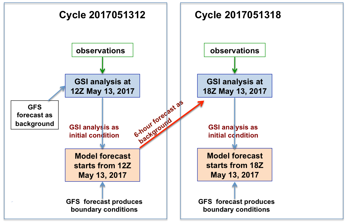
This exercise illustrate the basic structure and flow of a cycling data assimilation system, as shown in this chart (time doesn't match with the new case). It consists of running the GSI analysis with an ARW netcdf background field, and then the GSI analysis provides the initial fields for running a WRF-ARW forecast. The forecast output can be used as the GSI background for next GSI analysis.
The regional NAM BE is employed as the background error covariance and only conventional observations are assimilated in this example.
There are 4 steps in this GSI-ARW cycling data assimilation exercise:
- Step 1: GSI Data Analysis for 12Z of August 12, 2018. This step is similar to the online exercise ARW 3DVAR with conventional data (PrepBUFR)
- Step 2: WRF-ARW model forecast at 12Z of August 12, 2018, using the GSI analysis from step 1.
- Step 3: GSI Data Analysis for 18Z of August 12, 2018, using the 6-hour forecast output from step 2.
- Step 4: WRF-ARW model forecast at 18Z of August 12, 2018, using the GSI analysis from step 3.
GSI analysis at 12Z
GSI analysis at 12Z
GSI CYCLING RUN ARW BACKGROUND
GSI analysis at 12Z
For this step of GSI analysis at 12Z of August 12, 2018, we will use the GSI analysis output
wrf_inoutfrom the online exercise 03 ARW 3DVAR with conventional data (PrepBUFR) .
If you haven't practiced case 03, simply follow the steps in the above link to perform the GSI data assimilation and get the analysis.
Set up WRF-ARW run at 12Z
Set up WRF-ARW run at 12Z
GSI CYCLING RUN ARW BACKGROUND
Set up WRF-ARW run at 12Z
For this step of WRF-ARW run at 12Z of August 12, 2018, we will use the GSI analysis output
wrf_inoutfrom the online exercise 05 as the initial fields to launch 6-hour WRF forecast.
First, make sure you have a compiled code of the latest WRF-ARW code (V4.0). You can download the boundary condition for WRF from link .
Please follow the WRF tutorial and documents for the details of the WRF system application.
Here we provide the namelist file for reference of WRF run:
namelist.input
Running the ARW and checking the forecast results
The ARW can be run by creating a run script run_wrf.ksh and submitting it in the run directory:
bsub < run_wrf.kshIt will take a few minutes to finish. Once done, users should see the forecast files in each forecast hour from 12z to 20z like
wrfout_d01_2018-08-12_HH_00:00:00.The contents of this run directory are provided in the following list .
The ARW standard output file rsl.out.0000 is povided for reference.
GSI analysis at 18Z
GSI analysis at 18Z
GSI CYCLING RUN ARW BACKGROUND
GSI analysis at 18Z
For this step of GSI analysis at 18Z of August 12, 2018, we will use the 6-hour forecast output from the WRF run at 12Z as the background and conventional observations at 18Z. The steps to set up the GSI analysis is very similar to case 03, except for the background field and observations. The example run script can be found here.
Running the GSI run Script and checking the results
After GSI runs, a run directory will be created according to the path set in the variable
WORK_ROOT. The contents of this run directory are provided in the following list .The standard output file
stdoutand the fit files for this GSI run: temperature (fit_t1); wind (fit_w1); moisture (fit_q1).Convergence information (section 4.6 of the GSI User's Guide) is available in the file: fort.220
WRF-ARW run at 18Z
As a continued data assimilation run, the 18Z GSI analysis from the above step is then used as the initial field, together with the WRF background conditions at 18Z, to launch the WRF forecast at 18Z. The steps are very similar to the WRF run at 12Z and therefore not repeated here.
Case 7: 4D Hybrid EnVar Case
Case 7: 4D Hybrid EnVar Case
GSI 4D HYBRID FOR ARW USING GLOBAL ENSEMBLE FORECAST
Introduction
This exercise runs the GSI 4 Dimensional Ensemble-Variational (EnVar) hybrid analysis with the ARW background and conventional data at 18z August 12, 2018.
Please note the ARW background field is provided at three time levels in netcdf format from case 6, and the NAM BE is employed as the background error covariance in this experiment. The global ensemble files at three time levels are linked to run this GSI 4DEnVar hybrid test.Please check the Download Practice Data section if need to obtain the background, observation, and ensemble forecast files.
Setting up the Run Script for GSI 4D hybrid analysis
Setting up the Run Script for GSI 4D hybrid analysis
GSI 4D HYBRID FOR ARW USING GLOBAL ENSEMBLE FORECAST
Setting up the Run Script for GSI 4D hybrid analysis
Copy the sample run script
run_gsi_regional.kshfrom the practical case 3 (ARW 3DVAR with PrepBUFR) to a working directory and make the following modifications to run GSI 4D hybrid analysis:
- set the analysis time to
ANAL_TIME=2017051318- Set the name/path for the analysis run directory to
WORK_ROOT=${run directory}- Set the location of the ensemble files in the variable ENS_ROOT=...
- set the
BK_ROOTto where you store the background files, WRF forecast at 3 time levels- set the path to the background file at the analysis time
BK_FILE=${BK_ROOT}/wrfout_d01_2018-08-12_18:00:00- set to run 4D hybrid analysis
if_hybrid=Yes
if_4DEnVar=YesAs can be seen in the sample run script, for
${if_4DEnVar} = Yes, there are two additional background files at 1 hour before and after the analysis time, as specified in the variableBK_FILE_M1andBK_FILE_P1; there are also two additional sets of ensemble files before and after the analysis time, as specified in the variableENSEMBLE_FILE_mem_m1andENSEMBLE_FILE_mem_p1. Please make sure those variables setup right.An example of this run script is available from the link run_gsi_regional.ksh
Running the Script
Running the Script
GSI 4D HYBRID FOR ARW USING GLOBAL ENSEMBLE FORECAST
Running the Script
If you run on PBS system (Cheyenne), type:
qsub run_gsi_regional.ksh
to launch the job.
The progress of the job can be monitored by examining the tail of the standard out file in the run directory as specified in the variableWORK_ROOT:
tail stdoutWhen completed, the contents of this run directory are provided in the following list .
Results
Results
GSI 4D HYBRID FOR ARW USING GLOBAL ENSEMBLE FORECAST
Results
The standard output file
stdoutcontains the run diagnostics, such as convergence information, and observation distribution from the GSI run. Details of the standard output file are available in section 4.1 of the GSI User's Guide.Information about the use of observations by the analysis, and the corresponding innovations are available from the fit files (named
fort.2*). The fit files located in the run directory should agree with the following fit files for temperature (fit_t1); wind(fit_w1); moisture (fit_q1); surface pressure (fit_p1); and radiance (fit_rad1); and GPS (fort.212); and radar radial velocity(fort.209).Convergence information is available in the file: fort.220
Visualizing the Analysis
Use the same method as the practical case 3 (ARW 3DVAR) to make plots of the analysis increments. This time, plots will be made for the 2nd level (kmax=1) and level 21 (kmax=20). Once done pdf files GSI_Analysis_increment_1.pdf and GSI_Analysis_increment_20.pdf will be genera ted in the run directory. Compare these images with the reference solution [level 2 ] and [level 21].