Session 5: Trk&Int/Feature Relative
Session 5: Trk&Int/Feature Relative
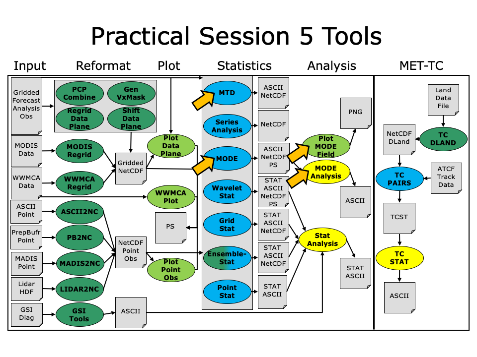
During the fifth METplus practical session, you will run the tools indicated below:
During this practical session, please work on the Session 5 exercises. You may navigate through this tutorial by following the arrows in the bottom-right or by using the left-hand menu navigation.
The MET Users Guide can be viewed here:
okular /classroom/wrfhelp/MET/8.0/met-8.0/doc/MET_Users_Guide.pdf &
MET Tool: TC-Pairs
MET Tool: TC-Pairs
TC-Pairs Tool: General
TC-Pairs Functionality
The TC-Pairs tool provides position and intensity information for tropical cyclone forecasts in Automated Tropical Cyclone Forecast System (ATCF) format. Much like the Point-Stat tool, TC-Pairs produces matched pairs of forecast model output and an observation dataset. In the case of TC-Pairs, both the model output and observational dataset (or reference forecast) must be in ATCF format. TC-Pairs produces matched pairs for position errors, as well as wind, sea level pressure, and distance to land values for each input dataset.
TC-Pairs input data format
As mentioned above, the input to TC-Pairs is two ATCF format files, in addition to the distance_to_land.nc file generated with the TC-Dland tool. The ATCF file format is a comma-separated ASCII file containing the following fields:
| Basin | basin | |
| CY | annual cyclone number (1-99) | |
| YYYYMMDDHH | Date - Time - Group | |
| TECHNUM/MIN | Objective sorting technique number, minutes in Best Track | |
| TECH | acronym for each objective technique | |
| TAU | forecast period | |
| LatN/S | Latitude for the date time group | |
| LonE/W | Longitude for date time group | |
| VMAX | Maximum sustained wind speed | |
| MSLP | Minimum sea level pressure | |
| TY | Highest level of tropical cyclone development | |
| RAD | wind intensity for the radii at 34, 50, 64 kts | |
| WINDCODE | radius code | |
| RAD1 | full circle radius of wind intensity, 1st quadrant wind intensity | |
| RAD2 | radius of 2nd quadrant wind intensity | |
| RAD3 | radius of 3rd quadrant wind intensity | |
| RAD4 | radius of 4th quadrant wind intensity | |
| ... |
These are the first 17 columns in the ATCF file format. MET-TC requires the input file has all 17 comma-separated columns present (although valid data is not required). For a full list of the columns as well as greater detail on the file format, see: http://www.nrlmry.navy.mil/atcf_web/docs/database/new/abdeck.txt
Model data must be run through a vortex tracking algorithm prior to becoming input for MET-TC. Running a vortex tracker is outside to scope of this tutorial, however a freely available and supported vortex tracking software is available at: http://www.dtcenter.org/HurrWRF/users/downloads/index.php
If users choose to use operational model data for input to MET-TC, all U.S. operational model output in ATCF format can be found at: ftp://ftp.nhc.noaa.gov/atcf/archive. Finally, the most common use of MET-TC is to use the best track analysis (used as observations) to generate pairs between the model forecast and the observations. Best track analyses can be found at the same link as the operational model output.
Open files /classroom/wrfhelp/MET/OBS/tc_data/aal182012.dat (model data) and /classroom/wrfhelp/MET/OBS/tc_data/bal182012.dat (BEST track). Take a look at the columns and gain familarity with ATCF format. These files are your input for TC-Pairs.
In addition to the files above, data from five total storms over hurricane seasons 2011-2012 in the AL basin will be used to run TC-Pairs. Rather than running a single storm, these storms were choosen to provide a larger sample size to provide more robust statistics.
- aal092011: Irene
- aal182011: Rina
- aal052012: Ernesto
- aal092012: Isaac
- aal182012: Sandy
TC-Pairs Tool: General
TC-Pairs Tool: General
TC-Pairs Tool: General
TC-Pairs Usage
View the usage statement for TC-Pairs by simply typing the following:
| Usage: tc_pairs | ||
| -adeck source | Input ATCF format track files | |
| -edeck source | Input ATCF format ensemble probability files | |
| -bdeck source | Input ATCF format observation (or reference forecast) file path/name | |
| -config file | Configuration file | |
| [-out_base] | path of output file base | |
| [-log_file] | name of log associated with tc_pairs output | |
| [-v level] | Level of logging (optional) |
At a minimum, the input ATCF format -adeck (or -edeck) source, the input ATCF format -bdeck source, and the configuration -config file must be passed in on the command line.
The -adeck, -edeck, and -edeck options can be set to either a specific file name or a top-level directory which will be searched for files ending in ".dat".
TC-Pairs Tool: Configure
TC-Pairs Tool: Configure
TC-Pairs Tool: Configure
Start by making an output directory for TC-Pairs and changing directories:
cd ${HOME}/metplus_tutorial/output/met_output/tc_pairs
Like the Point-Stat tool, the TC-Pairs tool is controlled by the contents of the configuration file passed to it on the command line. The default TC-Pairs configuration file may be found in the data/config/TCPairsConfig_default file.
The configurable items for TC-Pairs are used to specify which data are ingested and how the input data are filtered. The configurable items include specifications for the following:
- All model names to include in matched pairs
- Storms to include in verification: parsed by storm_id, basin, storm_name, cyclone
- Date/Time/Space restrictions: initialization time, valid time, lead time, masking
- User defined consensus forecasts
- Thresholds over watch/warning status of storm
The first step is to set-up the configuration file. Keep in mind, TC-Pairs should be run with the largest desired sample in mind to minimize re-running this tool! First, make a copy of the default:
Next, open up the TCPairsConfig_tutorial_run file for editing and modify it as follows:
Set:
basin = [ "AL" ];
To identify the models to we want to verify, as well as the basin. The three models identified are all U.S. operational models: HWRF, GFS (AVNO), and GFDL. Any field left blank will assume no restictions.
Set:
{
name = "CONS";
members = [ "HWRF", "AVNO", "GFDL" ];
required = [ false, false, false ];
min_req = 2;
}
];
To compute a user defined consensus named "CONS". The membership of the consensus are the three listed models, none are required, but 2 must be present to calculate the consensus.
Set:
To only keep pairs that are the intersection of the model forecast and observation.
Next, save the TCPairsConfig_tutorial_run file and exit the text editor.
TC-Pairs Tool: Run
TC-Pairs Tool: Run
TC-Pairs Tool: Run
Next, run TC-Pairs to compare all three ATCF forecast models specified in configuration file to the ATCF format best track analysis. Run the following command line:
-adeck /classroom/wrfhelp/MET/OBS/tc_data/aal*dat \
-bdeck /classroom/wrfhelp/MET/OBS/tc_data/bal*dat \
-config TCPairsConfig_tutorial_run \
-out tc_pairs \
-v 2
TC-Pairs is now grabbing the model data we requested in the configuration file, generating the consensus, and performing the additional filtering criteria. It should take only a few minutes to run. You should see several status messages printed to the screen to indicate progress.
If you are running many models over many storms/seasons, it is best to run TC-Pairs using a script to call TC-Pairs for each storm. This avoids potential memory issues when parsing very large datasets.
TC-Pairs Tool: Output
TC-Pairs Tool: Output
TC-Pairs Tool: Output
The output of TC-Pairs is an ASCII file containing matched pairs for each of the models requested. In this example, the output is written to the tc_pairs.tcst file as we requested on the command line. This output file is in TCST format, which is similar to the STAT output from the Point-Stat and Grid-Stat tools. For more header information on the TCST format, see section 19.2.3 of the MET User's Guide.
Remember to configure your text editor to NOT use dynamic word wrapping. The files will be much easier to read that way:
- In the kwrite editor, select Settings->Configure Editor, de-select Dynamic Word Wrap and click OK.
- In the vi editor, type the command :set nowrap. To set this as the default behavior, run the following command:
echo "set nowrap" >> ~/.exrc
Open tc_pairs.tcst
- Notice this is a simple ASCII file with rows for each matched pair for a single valid time..
- Any field that has A in the column name (such as AMAX_WIND, ALAT) indicate the model forecast.
- Any field that has B in the column name (such as BMAX_WIND, BLAT) indicate the observation field (Best Track).
- The TK_ERR, X_ERR, Y_ERR, ALTK_ERR, CRTK_ERR columns are calculated track error, X component position error, Y component postion error, along track error, and cross track error, respectively.
- Columns 34-63 are the 34-, 50-, and 64-kt wind radii for each quadrant.
MET Tool: TC-Stat
MET Tool: TC-Stat
TC-Stat Tool: General
TC-Stat Functionality
The TC-Stat tool reads the .tcst output file(s) of the TC-Pairs tool. This tools provides the ability to further filter the TCST output files as well as summarize the statistical information. The TC-Stat tool reads .tcst files and runs one or more analysis jobs on the data. TC-Stat can be run by specifying a single job on the command line or multiple jobs using a configuration file. The TC-Stat tool is very similar to the Stat-Analysis tool. The two analysis job types are summarized below:
- The filter job simply filters out lines from one or more TCST files that meet the filtering options specified.
- The summary job operates on one column of data from TCST file. It produces summary information for that column of data: mean, standard deviation, min, max, and the 10th, 25th, 50th, 75th, and 90th percentiles, independence time, and frequency of superior performance.
- The rirw job identifies rapid intensification or weakening events in the forecast and analysis tracks and applies categorical verification methods.
- The probrirw job applies probabilistic verification methods to evaluate probability of rapid inensification forecasts found in edeck's.
TC-Stat Usage
View the usage statement for TC-Stat by simply typing the following:
| Usage: tc_stat | ||
| -lookin path | TCST file or top-level directory containing TCST files (where TC-Pairs output resides). It allows the use of wildcards (at least one tcst file is required). | |
| [-out file] | Output path or specific filename to which output should be written rather than the screen (optional). | |
| [-log file] | Outputs log messages to the specified file | |
| [-v level] | Level of logging | |
| [-config config_file] | [JOB COMMAND LINE] (Note: "|" means "or") | ||
| [-config config_file] | TCStat config file containing TC-Stat jobs to be run. | |
| [JOB COMMAND LINE] | Arguments necessary to perform a TC-Stat job. |
At a minimum, you must specify at least one directory or file in which to find TCST data (using the -lookin path command line option) and either a configuration file (using the -config config_file command line option) or a job command on the command line.
TC-Stat Tool: Configure
TC-Stat Tool: Configure
TC-Stat Tool: Configure
Start by making an output directory for TC-Stat and changing directories:
cd ${HOME}/metplus_tutorial/output/met_output/tc_stat
The behavior of TC-Stat is controlled by the contents of the configuration file or the job command passed to it on the command line. The default TC-Stat configuration may be found in the data/config/TCStatConfig_default file. Make a copy of the default configuration file and make following modifications:
Open up the TCStatConfig_tutorial file for editing with your preferred text editor.
Set:
bmodel = [ "BEST" ];
event_equal = TRUE;
To only parse over two of the three model names in the tc_pairs.tcst file. The event_equal=TRUE flag will keep pairs that are in both HWRF and GFDL pairs.
Many of the filter options are left blank, indicating TC-Stat should parse over all available fields. You will notice many more available filter options beyond what was available with the TCPairsConfig.
Now, scroll all the way to the bottom of the TCStatConfig, and you will find the jobs[] section. Edit this section as follows:
TC-Stat: Run on TC-Pairs output
TC-Stat: Run on TC-Pairs output
TC-Stat: Run on TC-Pairs output
Run the TC-Stat using the following command:
-lookin ../tc_pairs/tc_pairs.tcst \
-config TCStatConfig_tutorial
Open the output file tc_stat.tcst. We can see that this filter job simply event equalized the two models specified in amodel.
Let's try to filter further, this time using the command line rather than the configuration file:
-job filter -lookin ../tc_pairs/tc_pairs.tcst \
-dump_row tc_stat2.tcst \
-water_only TRUE \
-column_str LEVEL HU,TS,TD,SS,SD \
-event_equal TRUE \
-match_points TRUE
Here, we ran a filter job at the command line: only keeping tracks over water (not encountering land) and with categories Hurricane (HU), Tropical Storm (TS), Tropical Depression (TD), Subtropical Storm (SS), and Subtropical Depression (SD).
Open the output file tc_stat2.tcst: notice fewer lines have been kept. Look at the "LEVEL" column ... note all the non-tropical and subtropical level classifications have been filtered out of the sample.
Also, find the columns ADLAND and BDLAND. All these values are now positive, meaning the tracks over land (negative values) have been filtered.
With the filtering jobs mastered, lets give the second type of job - summary jobs - a try!
TC-Stat: Run on TC-Pairs output
TC-Stat: Run on TC-Pairs output
TC-Stat: Run on TC-Pairs output
Now, we will run a summary job using TC-Stat on the command line using the following command:
-job summary -lookin ../tc_pairs/tc_pairs.tcst \
-amodel HWRF,GFDL \
-by LEAD,AMODEL \
-column TK_ERR \
-event_equal TRUE \
-out tc_stat_summary.tcst
Open up the file tc_stat_summary.tcst. Notice this output is much different from the filter jobs.
The track data is event equalized for the HWRF and GFDL models, and summary statistics are produced for the TK_ERR column for each model by lead time.
TC-Stat: Plotting with R
TC-Stat: Plotting with R
TC-Stat: Plotting with R
In this section, you will use the R statistics software package to produce a plot of a few results. R was introduced in practical session 1.
setenv MET_BASE $MET_INSTALL_DIR/share/met
Rscript $MET_BASE/Rscripts/plot_tcmpr.R
The TC-Stat tool can be called from the Rscript to do additional filter jobs on the TCST output from TC-Pairs. This can be done on the command line by calling a filter job (following tc-stat), or a configuraton file can be used to select filtering criteria. A default configuration file can be found in Rscripts/include/plot_tcmpr_config_default.R.
The configuration file also includes various plot types to generate: MEAN, MEDIAN, SCATTER, REFPERF, BOXPLOT, and RANK. All of the plot commands can be called on the command line as well as with the configuration file. Plots are configurable (title, colors, axis labels, etc) either by modifying the configuration file or setting options on the command line. To run from the command line:
-lookin ../tc_pairs/tc_pairs.tcst \
-filter "-amodel HWRF,CONS" \
-dep "TK_ERR" \
-series AMODEL HWRF,CONS \
-plot MEAN,BOXPLOT,RANK \
-outdir .
This plots the track error for two models: HWRF and CONS. CONS is the user defined consensus you generated in TC-Pairs.
Next, open up the output *png files:
okular TK_ERR_mean.png &
okular TK_ERR_rank.png &
The script produces the three plot types called in the configuration file:
- Boxplot showing distribution of errors for a homogeneous sample of the two models (TK_ERR_boxplot.png).
- Mean Errors with 95% CI for the same sample (TK_ERR_mean.png).
- Rank plot indicating performance of HWRF model relative to CONS (TK_ERR_rank.png).
Use Case: Track and Intensity
Use Case: Track and Intensity
METplus Use Case: Track and Intensity TCMPR (Tropical Cyclone Matched Pair) Plotter
This is a wrapper to the MET plot_tcmpr.R Rscript.
Based on your current mycustom.conf file settings you previously made, the track and intensity use cases should be able to run right now on the sample input data set dates. However, it is prudent to check the current use case you are about to run to make certain there are no unintended overriding settings. For example, do you have an unintended PROCESS_LIST setting that needs to be commented out, or is your OUTPUT_BASE set to a new location so you don't overwrite any previous output. Also, we are going to discuss an additional configuration file that is used to override the Rscripts default image size that will be generated.
Setup
Lets start by defining where to send the output by setting the OUTPUT_BASE configuration variable.
Edit Custom Configuration File
Define a unique directory under output that you will use for this use case.
Edit ${HOME}/METplus/parm/mycustom.conf
Change OUTPUT_BASE to contain a subdirectory specific to the Track and Intensity use case.
... other entries ...
OUTPUT_BASE = {ENV[HOME]}/metplus_tutorial/output/track_and_intensity
Review: Take a look at the following settings.
The default image resolution for the plot_tcmpr.R Rscript is set to 300, for print quality, but quite large for display purposes. The following is an R config file that is passed to the Rscript and changes the default and reduces the image size. It is a simple one line file, but go and take a look.
cat tcmpr_customize.conf
The plot_tcmpr.R script knows to read this tcmpr_customize.conf R config file since it is defined in METplus use case track_and_intensity.conf file as follows.
view the track_and_intensity.conf under the [config] section, with the following change.
NOTE: If you modify the CONFIG_FILE variable and leave it undefined (not set) CONFIG_FILE = , than no configuration file will be read by the R script and the default setting of 300 will be used.
These are some common settings for the track and intensity use case. These have already been defined in the track_and_intensity.conf file. If desired or needed, these can be overridden in this track and intesity use case conf files
TCMPR_DATA - the path to the input data, in this example, we are using the data in the TC_PAIRS_DIR directory.
MODEL_DATA_DIR - path to the METplus input data.
TRACK_DATA_DIR - path to the METplus input data.
Optional, Refer to section21.2.3 TC-Stat tool example of the MET Users Guide for a description of plot_tcmpr.R
If you wish, refer to Table 19.2 Format Information for TCMPR output line type, for a tabular description of the TC-Pairs output TCST format. After running this Track and Intensity example, you can view the TC-Pairs TCST output files generate by this example under your $HOME/METplus/metplus_tutorial/output/track_and_intensity/tc_pairs directory while comparing to the information in the table.
The tcmpr defaults are used for any conf settings left as, unset, For example as: XLAB =
The current settings in the conf files are ok and no changes are required. However, after running the exercise feel free to experiment with these settings.
The R script that Track and Intensity runs is located in the MET installation; share/met/Rscripts/plot_tcmpr.R. The usage statement with a short description of the options for plot_tcmpr.R can be obtained by typing: Rscript plot_tcmpr.R with no additional arguments. The usage statement can be helpful when setting some of the option in METplus, below is a description of these settings.
- CONFIG_FILE is a plotting configuration file
PREFIX is the output file name prefix.
TITLE overrides the default plot title. Bug: CAN_NOT_HAVE_SPACES
SUBTITLE overrides the default plot subtitle.
XLAB overrides the default plot x-axis label.
YLAB overrides the default plot y-axis label.
XLIM is the min,max bounds for plotting the X-axis.
YLIM is the min,max bounds for plotting the Y-axis.
FILTER is a list of filtering options for the tc_stat tool.
FILTERED_TCST_DATA_FILE is a tcst data file to be used instead of running the tc_stat tool.
DEP_VARS is a comma-separated list of dependent variable columns to plot.
SCATTER_X is a comma-separated list of x-axis variable columns to plot.
SCATTER_Y is a comma-separated list of y-axis variable columns to plot.
SKILL_REF is the identifier for the skill score reference.
LEGEND is a comma-separted list of strings to be used in the legend.
LEAD is a comma-separted list of lead times (h) to be plotted.
RP_DIFF is a comma-separated list of thresholds to specify meaningful differences for the relative performance plot.
DEMO_YR is the demo year
HFIP_BASELINE is a string indicating whether to add the HFIP baseline and which version (no, 0, 5, 10 year goal)
FOOTNOTE_FLAG to disable footnote (date).
PLOT_CONFIG_OPTS to read model-specific plotting options from a configuration file.
SAVE_DATA to save the filtered track data to a file instead of deleting it.
PLOT_TYPES- is a comma-separated list of plot types to create:
BOXPLOT, POINT, MEAN, MEDIAN, RELPERF, RANK, SKILL_MN, SKILL_MD
-for this example, set to MEAN,MEDIAN to generate MEAN and MEDIAN plots.
SERIES
- is the column whose unique values define the series on the plot,
optionally followed by a comma-separated list of values, including:
ALL, OTHER, and colon-separated groups.
SERIES_CI
- is a list of true/false for confidence intervals.
optionally followed by a comma-separated list of values, including:
ALL, OTHER, and colon-separated groups.
- is a comma-separated list of plot types to create:
Run METplus: Run Track and Intensity use case.
Examples: Run the track and intensity plotting script
Generates plots using the MET plot_tcmpr.R Rscript.
Example 1:
In this case, the track_and_intensity.conf file PLOT_TYPES is left unset, so the default BOXPLOT will be used.
Run the following command:
Example 2:
In this case, the tcmpr_mean_median.conf file PLOT_TYPES overrides the setting in track_and_intensity.conf to generate the MEAN,MEDIAN plots.
Run the following command:
The following directory lists the files generated from running these use cases:
AMAX_WIND-BMAX_WIND_median.png
AMSLP-BMSLP_mean.png
AMSLP-BMSLP_median.png
TK_ERR_boxplot.png
TK_ERR_mean.png
TK_ERR_median.png
To view the images generated by running these examples, use the display command.
cd to your OUTPUT_BASE/tcmpr_plots directory, depending on your setting it may be here.
display AMAX_WIND-BMAX_WIND_mean.png
MET Tool: Series-Analysis
MET Tool: Series-Analysis
Series-Analysis Tool: General
Series-Analysis Functionality
The Series-Analysis Tool accumulates statistics separately for each horizontal grid location over a series. Usually, the series is defined as a time series, however any type of series is possible, including a series of vertical levels. This differs from the Grid-Stat tool in that Grid-Stat computes statistics aggregated over a spatial masking region at a single point in time. The Series-Analysis Tool computes statistics for each individual grid point and can be used to quantify how the model performance varies over the domain.
Series-Analysis Usage
View the usage statement for Series-Analysis by simply typing the following:
| Usage: series_analysis | ||
| -fcst file_1 ... file_n | Gridded forecast files or ASCII file containing a list of file names. | |
| -obs file_1 ... file_n | Gridded observation files or ASCII file containing a list of file names. | |
| [-both file_1 ... file_n] | Sets the -fcst and -obs options to the same list of files (e.g. the NetCDF matched pairs files from Grid-Stat). |
|
| [-paired] | Indicates that the -fcst and -obs file lists are already matched up (i.e. the n-th forecast file matches the n-th observation file). |
|
| -out file | NetCDF output file name for the computed statistics. | |
| -config file | SeriesAnalysisConfig file containing the desired configuration settings. | |
| [-log file] | Outputs log messages to the specified file | |
| [-v level] | Level of logging (optional). | |
| [-compress level] | NetCDF compression level (optional). |
At a minimum, the -fcst, -obs (or -both), -out, and -config settings must be passed in on the command line. All forecast and observation fields must be interpolated to a common grid prior to running Series-Analysis.
Series-Analysis Tool: Configure
Series-Analysis Tool: Configure
Series-Analysis Tool: Configure
Start by making an output directory for Series-Analysis and changing directories:
cd ${HOME}/metplus_tutorial/output/met_output/series_analysis
The behavior of Series-Analysis is controlled by the contents of the configuration file passed to it on the command line. The default Series-Analysis configuration file may be found in the data/config/SeriesAnalysisConfig_default file. Prior to modifying the configuration file, users are advised to make a copy of the default:
The configurable items for Series-Analysis are used to specify how the verification is to be performed. The configurable items include specifications for the following:
- The forecast fields to be verified at the specified vertical level or accumulation interval.
- The threshold values to be applied.
- The area over which to limit the computation of statistics - as predefined grids or configurable lat/lon polylines.
- The confidence interval methods to be used.
- The smoothing methods to be applied.
- The types of statistics to be computed.
You may find a complete description of the configurable items in section 13.2.3 of the MET User's Guide. Please take some time to review them.
For this tutorial, we'll run Series-Analysis to verify a time series of 3-hour accumulated precipitation. We'll use GRIB1 for the forecast files and NetCDF for the observation files. Since the forecast and observations are different file formats, we'll specify the name and level information for them slightly differently.
Open up the SeriesAnalysisConfig_tutorial file for editing with your preferred text editor and edit it as follows:
- Set the fcst dictionary to
fcst = {
field = [
{
name = "APCP";
level = [ "A3" ];
}
];
}To request the GRIB abbreviation for precipitation (APCP) accumualted over 3 hours (A3).
- Delete obs = fcst; and insert
obs = {
field = [
{
name = "APCP_03";
level = [ "(*,*)" ];
}
];
}To request the NetCDF variable named APCP_03 where it's two dimensions are the gridded dimesnions (*,*).
- Set cat_thresh = [ >0.0, >=5.0 ];
To define the categorical thresholds of interest. By defining this at the top level of config file context, these thresholds will be applied to both the fcst and obs settings. - In the mask dictionary, set grid = "G212";
To limit the computation of statistics to only those grid points falling inside the NCEP Grid 212 domain. - Set block_size = 10000;
To process 10,000 grid points in each pass through the data. Setting block_size larger should make the tool run faster but use more memory. - In the output_stats dictionary, set
fho = [ "F_RATE", "O_RATE" ];
ctc = [ "FY_OY", "FN_ON" ];
cts = [ "CSI", "GSS" ];
mctc = [];
mcts = [];
cnt = [ "TOTAL", "RMSE" ];
sl1l2 = [];
pct = [];
pstd = [];
pjc = [];
prc = [];For each line type, you can select statistics to be computed at each grid point over the series. These are the column names from those line types. Here, we select the forecast rate (FHO: F_RATE), observation rate (FHO: O_RATE), number of forecast yes and observation yes (CTC: FY_OY), number of forecast no and observation no (CTC: FN_ON), critical success index (CTS: CSI), and the Gilbert Skill Score (CTS: GSS) for each threshold, along with the root mean squared error (CNT: RMSE).
Save and close this file.
Series-Analysis Tool: Run
Series-Analysis Tool: Run
Series-Analysis Tool: Run
First, we need to prepare our observations by putting 1-hourly StageII precipitation forecasts into 3-hourly buckets. Run the following PCP-Combine commands to prepare the observations:
pcp_combine -sum 00000000_000000 01 20050807_030000 03 \
sample_obs/ST2ml_3h/sample_obs_2005080703V_03A.nc \
-pcpdir /classroom/wrfhelp/MET/8.0/met-8.0/data/sample_obs/ST2ml
pcp_combine -sum 00000000_000000 01 20050807_060000 03 \
sample_obs/ST2ml_3h/sample_obs_2005080706V_03A.nc \
-pcpdir /classroom/wrfhelp/MET/8.0/met-8.0/data/sample_obs/ST2ml
pcp_combine -sum 00000000_000000 01 20050807_090000 03 \
sample_obs/ST2ml_3h/sample_obs_2005080709V_03A.nc \
-pcpdir /classroom/wrfhelp/MET/8.0/met-8.0/data/sample_obs/ST2ml
pcp_combine -sum 00000000_000000 01 20050807_120000 03 \
sample_obs/ST2ml_3h/sample_obs_2005080712V_03A.nc \
-pcpdir /classroom/wrfhelp/MET/8.0/met-8.0/data/sample_obs/ST2ml
pcp_combine -sum 00000000_000000 01 20050807_150000 03 \
sample_obs/ST2ml_3h/sample_obs_2005080715V_03A.nc \
-pcpdir /classroom/wrfhelp/MET/8.0/met-8.0/data/sample_obs/ST2ml
pcp_combine -sum 00000000_000000 01 20050807_180000 03 \
sample_obs/ST2ml_3h/sample_obs_2005080718V_03A.nc \
-pcpdir /classroom/wrfhelp/MET/8.0/met-8.0/data/sample_obs/ST2ml
pcp_combine -sum 00000000_000000 01 20050807_210000 03 \
sample_obs/ST2ml_3h/sample_obs_2005080721V_03A.nc \
-pcpdir /classroom/wrfhelp/MET/8.0/met-8.0/data/sample_obs/ST2ml
pcp_combine -sum 00000000_000000 01 20050808_000000 03 \
sample_obs/ST2ml_3h/sample_obs_2005080800V_03A.nc \
-pcpdir /classroom/wrfhelp/MET/8.0/met-8.0/data/sample_obs/ST2ml
Note that the previous set of PCP-Combine commands could easily be run by looping through times in a shell script or through a METplus use case! The MET tools are often run using a scripting language rather than typing individual commands by hand. You'll learn more about automation using the METplus python scripts.
Next, we'll run Series-Analysis using the following command:
-fcst /classroom/wrfhelp/MET/8.0/met-8.0/data/sample_fcst/2005080700/wrfprs_ruc13_03.tm00_G212 \
/classroom/wrfhelp/MET/8.0/met-8.0/data/sample_fcst/2005080700/wrfprs_ruc13_06.tm00_G212 \
/classroom/wrfhelp/MET/8.0/met-8.0/data/sample_fcst/2005080700/wrfprs_ruc13_09.tm00_G212 \
/classroom/wrfhelp/MET/8.0/met-8.0/data/sample_fcst/2005080700/wrfprs_ruc13_12.tm00_G212 \
/classroom/wrfhelp/MET/8.0/met-8.0/data/sample_fcst/2005080700/wrfprs_ruc13_15.tm00_G212 \
/classroom/wrfhelp/MET/8.0/met-8.0/data/sample_fcst/2005080700/wrfprs_ruc13_18.tm00_G212 \
/classroom/wrfhelp/MET/8.0/met-8.0/data/sample_fcst/2005080700/wrfprs_ruc13_21.tm00_G212 \
/classroom/wrfhelp/MET/8.0/met-8.0/data/sample_fcst/2005080700/wrfprs_ruc13_24.tm00_G212 \
-obs sample_obs/ST2ml_3h/sample_obs_2005080703V_03A.nc \
sample_obs/ST2ml_3h/sample_obs_2005080706V_03A.nc \
sample_obs/ST2ml_3h/sample_obs_2005080709V_03A.nc \
sample_obs/ST2ml_3h/sample_obs_2005080712V_03A.nc \
sample_obs/ST2ml_3h/sample_obs_2005080715V_03A.nc \
sample_obs/ST2ml_3h/sample_obs_2005080718V_03A.nc \
sample_obs/ST2ml_3h/sample_obs_2005080721V_03A.nc \
sample_obs/ST2ml_3h/sample_obs_2005080800V_03A.nc \
-out series_analysis_2005080700_2005080800_3A.nc \
-config SeriesAnalysisConfig_tutorial \
-v 2
The statistics we requested in the configuration file will be computed separately for each grid location and accumulated over a time series of eight three-hour accumulations over a 24-hour period. Each grid point will have up to 8 matched pair values.
Note how long this command line is. Imagine how long it would be for a series of 100 files! Instead of listing all of the input files on the command line, you can list them in an ASCII file and pass that to Series-Analysis using the -fcst and -obs options.
Series-Analysis Tool: Output
Series-Analysis Tool: Output
Series-Analysis Tool: Output
The output of Series-Analysis is one NetCDF file containing the requested output statistics for each grid location on the same grid as the input files.
You may view the output NetCDF file that Series-Analysis wrote using the ncdump utility. Run the following command to view the header of the NetCDF output file:
In the NetCDF header, we see that the file contains many arrays of data. For each threshold (>0.0 and >=5.0), there are values for the requested statistics: F_RATE, O_RATE, FY_OY, FN_ON, CSI, and GSS. The file also contains the requested RMSE and TOTAL number of matched pairs for each grid location over the 24-hour period.
Next, run the ncview utility to display the contents of the NetCDF output file:
Click through the different variables to see how the performance varies over the domain. Looking at the series_cnt_RMSEvariable, are the errors larger in the south eastern or north western regions of the United States?
Why does the extent of missing data increase for CSI for the higher threshold? Compare series_cts_CSI_gt0.0 to series_cts_CSI_ge5.0. (Hint: Find the definition of CSI in Appendix C of the MET User's Guide and look closely at the denominator.)
Try running Plot-Data-Plane to visualize the observation rate variable for non-zero precipitation (i.e. series_fho_O_RATE_gt0.0). Since the valid range of values for this data is 0 to 1, use that to set the -plot_range option.
Setting block_size to 10000 still required 3 passes through our 185x129 grid (= 23865 grid points). What happens when you increase block_size to 24000 and re-run? Does it run slower or faster?
Use Case: Feature Relative
Use Case: Feature Relative
METplus Use Case: Feature Relative (Series analysis by init)
Setup
In this exercise, you will perform a series analysis based on the init time of your sample data. This use case utilizes the MET tc_pairs, tc_stat, and series analysis tools, and the METplus wrappers: TcPairs, ExtractTiles, TcStat, and SeriesByInit. Please refer to the MET User's Guide for a description of the MET tools and section 3.5, 3.13, and 3.16 of the METplus 2.0.4 Users Guide for more details about the wrappers. Please note that the METplus User's Guide is a work-in-progress and may have missing content.
Open the mycustom.conf file in an editor of your choice:
Replace the following:
with this:
to keep this feature relative output separate from the other examples.
Using your custom configuration file that you created in the METplus: CUSTOM Configuration File Settings section and the Feature Relative use case configuration files that are distributed with METplus, you should be able to run the use case using the sample input data set without any other changes.
Review Use Case Configuration File: feature_relative.conf
View the file and study the configuration variables that are defined.
Note that variables in feature_relative.conf reference other variable you defined in your mycustom.conf configuration file.
For example:
This references OUTPUT_BASE which you set in your custom config file. METplus config variables can reference other config variables, even if they are defined in a config file that is read afterwards.
Run METplus
Run the following command:
You will see output streaming to your screen. This may take up to 4 minutes to complete. When it is complete, your prompt returns and you will see a line containing "INFO: INFO|Finished series analysis by init time" at the end of the screen output.
Review the Output Files
You should have output files in the following directories from the intermediate wrappers TcPairs, ExtractTiles, and TcStat, respectively:
${HOME}/metplus_tutorial/output/feature_relative/extract_tiles
${HOME}/metplus_tutorial/output/feature_relative/series_init_filtered
and the output of interest, from the SeriesByInit wrapper:
which has a directory corresponding to the date(s) of data in the data window:
and under that directory are subdirectories named by the storm:
${HOME}/metplus_tutorial/output/feature_relative/series_analysis_init/20141214_00/ML1200972014
${HOME}/metplus_tutorial/output/feature_relative/series_analysis_init/20141214_00/ML1200992014
${HOME}/metplus_tutorial/output/feature_relative/series_analysis_init/20141214_00/ML1201002014
${HOME}/metplus_tutorial/output/feature_relative/series_analysis_init/20141214_00/ML1201032014
${HOME}/metplus_tutorial/output/feature_relative/series_analysis_init/20141214_00/ML1201042014
${HOME}/metplus_tutorial/output/feature_relative/series_analysis_init/20141214_00/ML1201052014
${HOME}/metplus_tutorial/output/feature_relative/series_analysis_init/20141214_00/ML1201062014
${HOME}/metplus_tutorial/output/feature_relative/series_analysis_init/20141214_00/ML1201072014
${HOME}/metplus_tutorial/output/feature_relative/series_analysis_init/20141214_00/ML1201082014
${HOME}/metplus_tutorial/output/feature_relative/series_analysis_init/20141214_00/ML1201092014
${HOME}/metplus_tutorial/output/feature_relative/series_analysis_init/20141214_00/ML1201102014
and under each of those directories lies the files of interest:
FCST_ASCII_FILES_ML1200942014
series_TMP_Z2_FBAR.png
series_TMP_Z2_FBAR.ps
series_TMP_Z2_ME.png
series_TMP_Z2_ME.ps
series_TMP_Z2.nc
series_TMP_Z2_OBAR.png
series_TMP_Z2_OBAR.ps
series_TMP_Z2_TOTAL.png
series_TMP_Z2_TOTAL.ps
The ANLY_ASCII_FILES_ML########## (where ########## is the storm) is a text file that contains a list of the analysis data included in the series analysis. The FCST_ASCII_FILES_ML########## (where ########## is the storm) is a text file that contains a list of forecast data included in the series analysis.
The .nc files are the series analysis output generated from the MET series_analysis tool.
The .png and .ps files are graphics files that can be viewed using okular:
or
/bin/okular $HOME/metplus_tutorial/output/feature_relative/series_analysis_init/20141214_00/ML1200942014/series_TMP_Z2_FBAR.ps &
Note: the & is used to run this command in the background
Review the Log File
A log file is generated in your logging directory: ${HOME}/metplus_tutorial/output/feature_relative. The filename contains the timestamp corresponding to the current day. To view the log file:
Review the Final Configuration File
The final configuration file is $HOME/metplus_tutorial/output/grid_to_grid/metplus_final.conf. This contains all of the configuration variables used in the run.
Use Case: Feature Relative
Use Case: Feature Relative
METplus Use Case: Feature Relative (Series analysis by lead, by forecast hour grouping)
Setup
In this exercise, you will perform a series analysis based on the lead time (forecast hour) of your sample data and organize your results by forecast hour groupings. This use case utilizes the MET tc_pairs, tc_stat, and series analysis tools, and the METplus wrappers: TcPairs, ExtractTiles, TcStat, and SeriesByLead. Please refer to the MET User's Guide for a description of the MET tools and section 3.5, 3.13, and 3.16 of the METplus 2.0.4 Users Guide for more details about the wrappers. Please note that the METplus User's Guide is a work-in-progress and may have missing content.
Open the mycustom.conf file in an editor of your choice:
Replace the following:
with this:
to keep this feature relative output separate from the other examples.
Using your custom configuration file that you created in the METplus: CUSTOM Configuration File Settings section and the Feature Relative use case configuration files that are distributed with METplus, you should be able to run the use case using the sample input data set without any other changes.
Review Use Case Configuration File: series_by_lead_by_fhr_grouping.conf
View the file and study the configuration variables that are defined.
Note that variables in series_by_lead_fhr_grouping.conf reference other variable you defined in your mycustom.conf configuration file.
For example:
SERIES_LEAD_OUT_DIR = {OUTPUT_BASE}/series_analysis_lead
This references OUTPUT_BASE which you set in your custom config file. METplus config variables can reference other config variables, even if they are defined in a config file that is read afterwards.
Run METplus
Run the following command:
-c use_cases/feature_relative/examples/series_by_lead_by_fhr_grouping.conf \
-c mycustom.conf
You will see output streaming to your screen. This may take up to 3 minutes to complete. When it is complete, your prompt returns.
Review the Output Files
You should have the following output directories that result from running the wrappers TcPairs, ExtractTiles, and TcStat, respectively:
${HOME}/metplus_tutorial/output/series_by_lead_fhr_grouping/track_data_atcf_pairs
${HOME}/metplus_tutorial/output/series_by_lead_fhr_grouping/extract_tiles
${HOME}/metplus_tutorial/output/series_by_lead_fhr_grouping/series_lead_filtered
and the output directory of interest, from the SeriesByLead wrapper:
which has a directory corresponding to the date(s) of data in the time window:
and under that directory are subdirectories named by the storm:
${HOME}/metplus_tutorial/output/series_by_lead_fhr_grouping/series_analysis_lead/20141214_00/ML1200972014
${HOME}/metplus_tutorial/output/series_by_lead_fhr_grouping/series_analysis_lead/20141214_00/ML1200992014
${HOME}/metplus_tutorial/output/series_by_lead_fhr_grouping/series_analysis_lead/20141214_00/ML1201002014
${HOME}/metplus_tutorial/output/series_by_lead_fhr_grouping/series_analysis_lead/20141214_00/ML1201032014
${HOME}/metplus_tutorial/output/series_by_lead_fhr_grouping/series_analysis_lead/20141214_00/ML1201042014
${HOME}/metplus_tutorial/output/series_by_lead_fhr_grouping/series_analysis_lead/20141214_00/ML1201052014
${HOME}/metplus_tutorial/output/series_by_lead_fhr_grouping/series_analysis_lead/20141214_00/ML1201062014
${HOME}/metplus_tutorial/output/series_by_lead_fhr_grouping/series_analysis_lead/20141214_00/ML1201072014
${HOME}/metplus_tutorial/output/series_by_lead_fhr_grouping/series_analysis_lead/20141214_00/ML1201082014
${HOME}/metplus_tutorial/output/series_by_lead_fhr_grouping/series_analysis_lead/20141214_00/ML1201092014
${HOME}/metplus_tutorial/output/series_by_lead_fhr_grouping/series_analysis_lead/20141214_00/ML1201102014
and under each of those directories lies the files of interest:
Day1
Day2
Day3
Day4
series_animate
The directories Dayn contain the following files:
series_F000_to_F018_TMP_Z2_ME.png
series_F000_to_F018_TMP_Z2_OBAR.ps
FCST_FILES_F000_to_F018
series_F000_to_F018_TMP_Z2_ME.ps
series_F000_to_F018_TMP_Z2_TOTAL.png
series_F000_to_F018_TMP_Z2_FBAR.png
series_F000_to_F018_TMP_Z2.nc
series_F000_to_F018_TMP_Z2_TOTAL.ps
series_F000_to_F018_TMP_Z2_FBAR.ps
series_F000_to_F018_TMP_Z2_OBAR.png
The ANLY_FILES_F000_to_F018 is a text file that contains a list of the data that is included in the series analysis.
The .nc files are the series analysis output generated from the MET series_analysis tool.
The .png and .ps files are graphics files that can be viewed using okular:
or
/bin/okular ${HOME}/metplus_tutorial/output/series_by_lead_fhr_grouping/series_analysis_lead/Day1/series_F000_to_F018_TMP_Z2_FBAR.ps &
Note: the & is used to run this command in the background
The series_animate directory contains the gif images of the animations:
series_animate_TMP_Z2_FBAR.gif
series_animate_TMP_Z2_ME.gif
series_animate_TMP_Z2_OBAR.gif
series_animate_TMP_Z2_TOTAL.gif
To watch the animations, cd to ${HOME}/metplus_tutorial/output/series_by_lead_fhr_grouping/series_animate, enter the following:
firefox ${HOME}/metplus_tutorial/output/series_by_lead_fhr_grouping/series_animate/series_animate_TMP_Z2_ME.gif
firefox ${HOME}/metplus_tutorial/output/series_by_lead_fhr_grouping/series_animate/series_animate_TMP_Z2_OBAR.gif
Review the Log File
A log file is generated in your logging directory: ${HOME}/metplus_tutorial/output/series_by_lead_fhr_grouping. The filename contains the timestamp corresponding to the current day. To view the log file:
Review the Final Configuration File
The final configuration file is $HOME/metplus_tutorial/output/grid_to_grid/metplus_final.conf. This contains all of the configuration variables used in the run.
METviewer
METviewer
METviewer: General
METviewer Overview
METviewer is a database and display system for storing and plotting data from the MET .stat and MODE _obj.txt files. It is used heavily within the DTC and by NOAA-GSD and NOAA-EMC. While its distribution is limited, it is available to the community through a Docker container. For more information, please see:
- Numerical Weather Prediction (NWP) Containers DTC tutorial to run WPS, GSI, WRF, UPP, MET, and METviewer with containers.
- METviewer Source Code GitHub repository (https://github.com/NCAR/metviewer)
- METviewer Container GitHub repository (https://github.com/NCAR/container-dtc-metviewer)
Here, we will use the publicly available version of METviewer running at NCAR to demonstrate the METviewer webapp.
METviewer reads MET verification statistics from a database and creates plots using the R statistical package. The tool includes a web application that can be accessed from a web browser to create a single plot. The specification for each plot is built using a series of controls and then serialized into XML. For each plot, METviewer generates a SQL query, an R script to create the plot, a flat file containing the data that will be plotted and the plot itself.
METviewer Web Application
The following example can be run using the METviewer instance located at the link below. It is recommended to move the new tab into a new browser window, so that you can view both the example instructions and the METviewer web application side-by-side.
The following pages have instructions for generating two different types of plots:
- A threshold series plot of Accuracy (ACC) and Critical Success Index (CSI)
- A forecast lead time box plot series of MODE object area distributions
Please be sure to follow these instructions in order.
METviewer: Time Series of Categorical Statistics Plot
METviewer: Time Series of Categorical Statistics Plot
METviewer: Time Series of Categorical Statistics Plot
The following list shows the setting name and the setting value for each of the controls on the web application. Please go through them in order, starting at the top, setting and checking the controls as suggested. The settings that you need to change are marked in blue. The settings are grouped according to the areas on the web app. If you need more information about the controls, please click the little i in a circle to the right of METviewer 2.9 at the very top of the page. This will take you to the METviewer documentation.
- Database: Click on the box named Select databases and from the Verification group, select mv_met_tutorial
To make a plot with sample tutorial data. - Tab: Series - Create a time-series (as we will do here) or threshold-series line plot. The different tabs correspond to the types of plots that METviewer can generate, such as box plots, bar plots, histograms, and ensemble plots.
- Plot Data: Stat - Plot traditional statistics as opposed to MODE object attributes.
- Y1 Axis variables - These controls specify the statistics and curves for the Y1 axis of the plot.
Y1 Dependent (Forecast) Variables - pairs of forecast variables and statistics to be plotted- Click dropdown list and select: APCP_03 - to select 3-hourly Accumulated Precipitation
- Click Select attribute stat dropdown list and select: ACC and CSI - to plot Accuracy and Critical Success Index
Y1 Series Variables - specifies the lines on the plot for each dependent variable
- Click the dropdown list and select: MODEL
- Click the Select value dropdown list and select: QPF - output for only one model is present
- Next, click the + Series Variable button, click the dropdown list, and select: FCST_THRESH
- Click the Select value dropdown list and select: >0.0, >2.54, and >6.35 - to plot statistics for 3 categorical thresholds
- Y2 Axis Tab - these controls specify the statistics and curves for the Y2 axis of the plot; it is not used in this demonstration
- Fixed Values - field/value pairs that are held constant for all data on the plot
- Click the +Fixed Value button - to add a fixed value selection option
- Click the dropdown list and select VX_MASK
- Click the Select value dropdown list and select: FULL - to plot data for FULL model domain (the only one present in this dataset)
- Independent Variable - the x-axis field and values over which the data are displayed on the plot
- Click the dropdown list and select FCST_LEAD
- Click the Select value dropdown list and click the Check all option - to select all items
- Statistics -
The Summary radio button tells MET to plot the mean or median of the statistics pulled directly from the database.
The Aggregation statistics radio button tells METviewer to aggregate contingency table counts or partial sums and compute aggregate summary statistics and confidence intervals.
Use the default Summary radio button selection.
- Series Formatting - settings to control colors, line types, plotting symbols, and confidence intervals
- There should be settings for 6 lines: 3 lines for ACC followed by 3 lines for CSI. In the Line Color column:
- Set the 1st and 4th lines to the same RED color.
- Set the 2nd and 5th lines to the same GREEN color.
- Set the 3rd and 6th lines to the same BLUE color.
- In the Series Line Type column:
- Set the 4th, 5th, and 6th to Dashed.
- Plot Formatting - settings that control the appearance of the plot, along with several miscellaneous features
- On the Titles & Labels tab, set Plot Title to ACC / CSI vs. Lead Time
- On the Titles & Labels tab, set X label to Forecast Lead
- On the Titles & Labels tab, set Y1 label to ACC / CSI
- On the Common tab, select Display Number of Stats
- Click the Generate Plot button at the top of the page - to submit your plot request to the METviewer plotting engine.
METviewer: Time Series of Categorical Statistics Plot Output
METviewer: Time Series of Categorical Statistics Plot Output
METviewer: Time Series of Categorical Statistics Plot Output
If you successfully followed the instructions on the previous page, you should see a plot appear in the in the plot tab of the METviewer window. Your plot should look like this. And here is the corresponding plot xml.
Studying the plot shows that the Critical Success Index (CSI) decreases for higher thresholds, as if often the case. This suggests that the forecast models have more skill at lower precipitation thresholds. This contrasts with the story told by the accuracy statistic, which increases as the threshold increases. This can be explained by the simplicity of the accuracy statistic, and the effect that always predicting no event can have for extreme events.
The following section discusses the output that METviewer generates for each plot. Click through the tabs above the METviewer plot to examine each:
- XML Tab: When the Generate Plot button is clicked, the web application serializes the information in the web page controls into an XML document and sends it across the internet to METviewer. This XML document can be used to generate a plot directly from METviewer using the command line interface, also called the batch engine. The batch engine can create many plots from a single XML document, using only small changes. Thus, a good way to use the METviewer web application is to "design" plots and then take the XML for the plot and extend it to create many different plots.
- Log Tab: The METviewer plot engine generates status output as it runs, and this information can be useful for finding problems.
- R script Tab: METviewer uses the R statistics package to generate plots by constructing an R script and running it in R. The R script that is constructed can be saved and modified if the users would like to make changes to the plot that are not supported in METviewer.
- R data Tab: Along with the R script generated by METviewer for the plot, the plot data is stored in a file that is read when the plot is generated in R. This file can be useful for problem solving, since it shows all of the data used in the plot and can be loaded directly into R for analysis.
- SQL Tab: All of the MET verification statistics output is stored in a database, which METviewer searches when it generates a plot. The SQL generated by METviewer to gather the data for a plot can be viewed, in case the user wants to explore or debug using the SQL directly.
METviewer: Object Based Attribute Area Box Plot
METviewer: Object Based Attribute Area Box Plot
METviewer: Object Based Attribute Area Box Plot
For the next plot, you'll try out the XML upload feature. Each plot created by METviewer corresponds to an XML file that defines the plot. In this example, you'll load the XML from a previous plot and regenerate it.
- Right click on this XML file, select the Save Link As option, and save the file to your machine.
- In the METviewer window, click on the Load XML button in the top-right corner.
- In the Upload plot XML file dialog box, click the Browse button, and navigate the location of the XML file.
- Select the XML file, click the Open button, and then the OK button.
- METviewer will now populate all of the selections with those specified in that XML file.
- Lastly, click the Generate Plot button at the top of the page to create the image. Your plot should look like this.
This plot shows the area of MODE objects defined for 1-hourly accumulated precipitation thresholded at 0.1 inch. The data has been filtered down to the 00Z initialization and the areas are plotted by lead time. Each lead time has 3 boxplots: core1 in red, core2 in blue, and the observations in gray. The numbers in black across the top show the number of objects plotted for each lead time.
Note that we have only plotted the observations once since they should be the same for both models. Look in the Series Formatting section at the bottom of the METviewer webapp in the Hide column to see that we're hiding the 4th series titled core2_hwt APCP_01 AREA_OSA. Also note that in the Legend Text column, we've specified our own strings rather than using the METviewer defaults.
The XML Upload feature of METviewer is very powerful and has saved users a lot of time by uploading previous work rather than starting from scratch each time.
Feel free to experiment with METviewer and make additional plots.
End of Practical Session 5
End of Practical Session 5
End of Practical Session 5
Congratulations! You have completed Session 5!
Tutorial Survey
Tutorial Survey
METplus Tutorial Survey
Thank you for your time and attention. We really enjoyed teaching you about METplus.
Please remember to fill out the METplus Tutorial Survey to receive your certificate of completion.
If you have more questions in your use of MET, please:
- Refer to the MET User's Guide and Presentations.
- Refer to the MET Online Tutorial.
- Refer to the Known Issues Section of the MET website.
- Use a search engine to search for met_help followed by your question, issue, or error message.
- Browse through the MET-Help email archive.
- Email us directly at met_help@ucar.edu.
Now go out there and Verify!