METplus Examples of Probabilistic Forecast Verification

METplus Examples of Probabilistic Forecast Verification

The following two examples show a generalized method for calculating probabilistic statistics: one for a MET-only usage, and the same example but utilizing METplus wrappers. These examples are not meant to be completely reproducible by a user: no input data is provided, commands to run the various tools are not given, etc. Instead, they serve as a general guide of one possible setup among many that produce probabilistic statistics.

If you are interested in reproducible, step-by-step examples of running the various tools of METplus, you are strongly encouraged to review the METplus online tutorial that follows this statistical tutorial, where data is made available to reproduce the guided examples.

In order to better understand the delineation between METplus, MET, and METplus wrappers which are used frequently throughout this tutorial but are NOT interchangeable, the following definitions are provided for clarity:

• METplus is best visualized as an overarching framework with individual components. It encapsulates all of the repositories: MET, METplus wrappers, METdataio, METcalcpy, and METplotpy.
• MET serves as the core statistical component that ingests the provided fields and commands to compute user-requested statistics and diagnostics.
• METplus wrappers is a suite of Python wrappers that provide low-level automation of MET tools and plotting capability. While there are examples of calling METplus wrappers without any underlying MET usage, these are the exception rather than the rule.

MET Example of Probabilistic Forecast Verification

Here is an example that demonstrates probabilistic forecast verification using MET.

For this example, we will use two tools: Gen-Ens-Prod, which will be used to create uncalibrated probability forecasts, and Grid-Stat, which will verify the forecast probabilities against an observational dataset. The “uncalibrated” term means that the probabilities gathered from Gen-Ens-Prod may be biased and will not perfectly reflect the true probabilities of the forecasted event. To avoid complications with assuming gaussian distributions on non-gaussian variable fields (i.e. precipitation), we’ll verify the probability of a CONUS 2 meter temperature field from a global ensemble with 5 members with a threshold of greater than 10 degrees Celsius.

Starting with the general Gen-Ens-Prod configuration file, the following would resemble the minimum necessary settings/changes for the ens dictionary:

We can see right away that Gen-Ens-Prod is different from most MET tools; it utilizes only one dictionary to process fields (as opposed to the typical forecast and observation fields). This is by design and follows the guidance that Gen-Ens-Prod generates ensemble products, rather than verifying ensemble forecasts (which is left for Ensemble-Stat). Even with this slight change, the name and level entries are still set the same as they would be in any MET tool; that is, according to the information in the input files (e.g., a variable field named TMP on the second vertical level). The cat_thresh entry reflects an interest in 2 meter temperatures greater than 10 degrees Celsius. We’ve also included a convert function which will convert the field from its normal output of Kelvin to degrees Celsius. If you’re interested in learning more about this tool, including in-depth explanations of the various settings, please review the MET User’s Guide entry for Gen-Ens-Prod or get a hands-on experience with the tool in the METplus online tutorial.

Let’s also utilize the regrid dictionary, since we are only interested in CONUS and the model output is global:

More discussion on how to properly use the regrid dictionary and all of its associated settings can be found in the MET User’s Guide.

All that’s left before running the tool is to set up the ensemble_flag dictionary correctly:

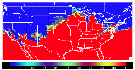
In the first half of this example, we have told MET to create a CONUS 2 meter temperature field count from 0.0 to 1.0 at each grid point representing how many of the ensemble members forecast a temperature greater than 10 degrees Celsius. So with this configuration file we’ll create a probability field based on ensemble member agreement and disagreement.

The output from Gen-Ens-Prod is a netCDF file whose content would contain a variable field as described above. It should look something like the following:

With this new MET field output, we can verify this uncalibrated probabilistic forecast for 2 meter temperatures greater than 10 degrees Celsius against an observation dataset in Grid-Stat.

Now for the actual verification and statistical generation we turn to Grid-Stat. Starting with the general Grid-Stat configuration file, let’s review how we might set the fcst dictionary:

In this example we see the name of the variable field from the Gen-Ens-Prod tool’s netCDF output file, TMP_Z2_ENS_FREQ_gt10, set as the forecast field name. The prob setting informs MET to process the field as probabilistic data, which requires an appropriate categorical threshold creation. Using “==0.1” means MET will create 10 bins from 0 to 1, each with a width of 0.1. Recall from previous discussion on how MET evaluates probabilities that MET will use the midpoints of each of these bins to evaluate the forecast. Since the forecast data probabilistic resolution is 0.1, the use of 0.05 as the evaluation increment is reasonable. 

Now let’s look at a possible setup for the obs dictionary:

Notice that we’ve used the convert function again to change the original Kelvin field to degrees Celsius, along with the appropriate variable field name and second vertical level request. For the threshold we re-use the same value that was originally used to create the forecast probabilities, greater than 10 degrees Celsius. This matching value is important as any other comparison would mean an evaluation between two inconsistent fields.

Since the forecast and observation fields are on different grids, we’ll utilize the regrid dictionary once again to place everything on the same evaluation gridspace:

Finally, we choose the appropriate flags in the output_flag dictionary to gain the probabilistic statistics:

With a successful run of MET, we should find a .stat file with two rows of data; one for the PCT line type that will provide information on the specific counts of observations that fell into each of the forecast’s probability bins, and one for the PSTD line type which has some of the probabilistic measures we discussed in this chapter. The content might look similar to the following:

Note that the rows have been truncated and would normally hold more information to the left of the FCST_THRESH entry. But from this snippet we see that there were 103,936 matched pairs for the comparison, with PCT line type showing many of the observations falling in the “no” category of the 0 to 0.1 bin and the “yes” category of the 0.9 to 1.0 bin. In fact, less than seven percent of the matched pairs fell into categories outside of these two. This distribution tells us that the model was very confident in its probabilities, supported by the observations. This is reflected in the outstanding statistical values of the PSTD line type, including a 0.0019261 Reliability value (recall that a zero is ideal and indicates less differences between the average forecast probability and the observed average frequency) and a near-perfect Brier score of 0.019338 (0 being a perfect score). There is some room for improvement, as reflected in a 0.231 Resolution value (remember that this is the measure of the forecast’s ability to resolve different observational distributions given a change in the forecast value, and a larger value is desirable). For a complete list of all of the statistics given in these two line types, review the MET User’s Guide entries for the PCT and PSTD line types.

METplus Wrapper Example of Probabilistic Forecast Verification

To achieve the same success as the previous example, but utilizing METplus wrappers instead of MET, very few adjustments would need to be made. In fact, approaching this example utilizing the wrappers simplifies the problem, as one configuration file can be used to generate the desired output from both tools.

Starting with variable fields, we would need to set the _VAR1 settings appropriately. Since we are calling two separate tools, it would be best practice to utilize the individual tool’s variable field settings, as seen below:

You can see how the GenEnsProd field variables start with the prefix ENS_, and the GridStat wrapper field variables have _GRID_STAT_ in their name. Those GridStat field settings are also clearly separated into forecast (FCST_) and observation (OBS_) options. Note how from the MET-only approach we have simply changed what the setting name is, but the same values are utilized, all in one configuration file.

To recreate the regridding aspect of the MET example, we would call the wrapper-appropriate regridding options:

Because the loop/timing information is controlled inside the configuration file for METplus wrappers (as opposed to MET’s non-looping option), that information must also be set accordingly. This is also an appropriate time to set up the calls to the wrappers in the desired order:

Now a one time loop will be executed with a forecast lead time of 24 hours, matching the forecast and observation datasets’ relationship.

One part that needs to be done carefully is the input directory and file name template for GridStat. This is because we are relying on the output from the previous wrapper, GenEnsProd, and need to set the variable accordingly. As long as the relative value is used, this process becomes much simpler, as shown:

These commands will tie the input for GridStat to wherever the output from GenEnsProd was set.

Finally we set up the correct output requests for each of the tools:

And with a successful run of METplus we would arrive at the same output as we obtained from the MET-only example. This example once again highlights the usefulness of METplus wrappers in chaining multiple tools together in one configuration file.