Session 3: Analysis Tools
Session 3: Analysis Tools
METplus Practical Session 3
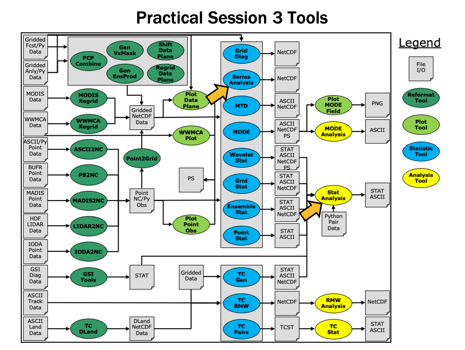
During this practical session, you will run the tools indicated below:
 You may navigate through this tutorial by following the links at the bottom of each page or by using the menu navigation.
Since you already set up your runtime enviroment in Session 1, you should be ready to go! To be sure, run through the following instructions to check that your environment is set correctly.
Prerequisites: Verify Environment is Set Correctly
Before running the tutorial instructions, you will need to ensure that you have a few environment variables set up correctly. If they are not set correctly, the tutorial instructions will not work properly.
EDIT AFTER COPYING and BEFORE HITTING RETURN!
source METplus-5.0.0_TutorialSetup.sh
echo ${METPLUS_BUILD_BASE}
echo ${MET_BUILD_BASE}
echo ${METPLUS_DATA}
ls ${METPLUS_TUTORIAL_DIR}
ls ${METPLUS_BUILD_BASE}
ls ${MET_BUILD_BASE}
ls ${METPLUS_DATA}
METPLUS_BUILD_BASE is the full path to the METplus installation (/path/to/METplus-X.Y)
MET_BUILD_BASE is the full path to the MET installation (/path/to/met-X.Y)
METPLUS_DATA is the location of the sample test data directory
ls ${METPLUS_BUILD_BASE}/ush/run_metplus.py
See the instructions in Session 1 for more information.
You are now ready to move on to the next section.
MET Tool: Stat-Analysis
MET Tool: Stat-Analysis
Stat-Analysis Tool: General
Stat-Analysis Functionality
The Stat-Analysis tool reads the ASCII output files from the Point-Stat, Grid-Stat, Wavelet-Stat, and Ensemble-Stat tools. It provides a way to filter their STAT data and summarize the statistical information they contain. If you pass it the name of a directory, Stat-Analysis searches that directory recursively and reads any .stat files it finds. Alternatively, if you pass it an explicit file name, it'll read the contents of the file regardless of the suffix, enabling it to the optional _LINE_TYPE.txt files. Stat-Analysis runs one or more analysis jobs on the input data. It can be run by specifying a single analysis job on the command line or multiple analysis jobs using a configuration file. The analysis job types are summarized below:
- The filter job simply filters out lines from one or more STAT files that meet the filtering options specified.
- The summary job operates on one column of data from a single STAT line type. It produces summary information for that column of data: mean, standard deviation, min, max, and the 10th, 25th, 50th, 75th, and 90th percentiles.
- The aggregate job aggregates STAT data across multiple time steps or masking regions. For example, it can be used to sum contingency table data or partial sums across multiple lines of data. The -line_type argument specifies the line type to be summed.
- The aggregate_stat job also aggregates STAT data, like the aggregate job above, but then derives statistics from that aggregated STAT data. For example, it can be used to sum contingency table data and then write out a line of the corresponding contingency table statistics. The -line_type and -out_line_type arguments are used to specify the conversion type.
- The ss_index job computes a skill-score index, of which the GO Index (go_index) is a special case. The GO Index is a performance metric used primarily by the United States Air Force.
- The ramp job processes a time series of data and identifies rapid changes in the forecast and observation values. These forecast and observed ramp events are used populate a 2x2 contingency table from which categorical statistics are derived.
Stat-Analysis Usage
View the usage statement for Stat-Analysis by simply typing the following:
| Usage: stat_analysis | ||
| -lookin path | Space-separated list of input paths where each is a _TYPE.txt file, STAT file, or directory which should be searched recursively for STAT files. Allows the use of wildcards (required). | |
| [-out filename] | Output path or specific filename to which output should be written rather than the screen (optional). | |
| [-tmp_dir path] | Override the default temporary directory to be used (optional). | |
| [-log file] | Outputs log messages to the specified file | |
| [-v level] | Level of logging | |
| [-config config_file] | [JOB COMMAND LINE] (Note: "|" means "or") | ||
| [-config config_file] | STATAnalysis config file containing Stat-Analysis jobs to be run. | |
| [JOB COMMAND LINE] | All the arguments necessary to perform a single Stat-Analysis job. See the MET Users Guide for complete description of options. |
At a minimum, you must specify at least one directory or file in which to find STAT data (using the -lookin path command line option) and either a configuration file (using the -config config_file command line option) or a job command on the command line.
Configure
Configure
Stat-Analysis Tool: Configure
cd ${METPLUS_TUTORIAL_DIR}/output/met_output/stat_analysis
The behavior of Stat-Analysis is controlled by the contents of the configuration file or the job command passed to it on the command line. The default Stat-Analysis configuration may be found in the data/config/StatAnalysisConfig_default file.
You will see that most options are left blank, so the tool will use whatever it finds or whatever is specified in the command or job line. If you go down to the jobs[] section you will see a list of the jobs run for the test scripts.
"-job aggregate -line_type CTC -fcst_thresh >273.0 -vx_mask FULL -interp_mthd NEAREST",
"-job aggregate_stat -line_type CTC -out_line_type CTS -fcst_thresh >273.0 -vx_mask FULL -interp_mthd NEAREST"
];
The first job listed above will select out only the contingency table count lines (CTC) where the threshold applied is >273.0 over the FULL masking region. This should result in 2 lines, one for pressure levels P850-500 and one for pressure P1050-850. So this job will be aggregating contingency table counts across vertical levels.
The second job listed above will perform the same aggregation as the first. However, it'll dump out the corresponding contingency table statistics derived from the aggregated counts.
Run on Point-Stat output
Run on Point-Stat output
Stat-Analysis Tool: Run on Point-Stat output
-config STATAnalysisConfig_tutorial \
-lookin ../point_stat \
-v 2
The output for these two jobs are printed to the screen.
-config STATAnalysisConfig_tutorial \
-lookin ../point_stat \
-v 2 \
-out aggr_ctc_lines.out
The output was written to aggr_ctc_lines.out. We'll look at this file in the next section.
-lookin ../point_stat \
-v 2 \
-job aggregate \
-line_type CTC \
-fcst_thresh ">273.0" \
-vx_mask FULL \
-interp_mthd NEAREST
Note that we had to put double quotes (") around the forecast theshold string for this to work.
-lookin ../point_stat \
-v 2 \
-job aggregate \
-line_type CTC \
-fcst_thresh ">273.0" \
-vx_mask FULL \
-interp_mthd NEAREST \
-dump_row aggr_ctc_job.stat \
-out_stat aggr_ctc_job_out.stat
Output
Output
Stat-Analysis Tool: Output
On the previous page, we generated the output file aggr_ctc_lines.out by using the -out command line argument.
This file contains the output for the two jobs we ran through the configuration file. The output for each job consists of 3 lines as follows:
- The JOB_LIST line contains the job filtering parameters applied for this job.
- The COL_NAME line contains the column names for the data to follow in the next line.
- The third line consists of the line type generated (CTC and CTS in this case) followed by the values computed for that line type.
-lookin ../point_stat/point_stat_run2_360000L_20070331_120000V.stat \
-v 2 \
-job aggregate \
-fcst_var TMP \
-fcst_lev Z2 \
-vx_mask EAST -vx_mask WEST \
-interp_pnts 1 \
-line_type CTC \
-fcst_thresh ">278.0"
This job should aggregate 2 CTC lines for 2-meter temperature across the EAST and WEST regions.
-
Do the same aggregation as above but for the 5x5 interpolation output (i.e. 25 points instead of 1 point).
-
Do the aggregation listed in (1) but compute the corresponding contingency table statistics (CTS) line. Hint: you will need to change the job type to aggregate_stat and specify the desired -out_line_type.
How do the scores change when you increase the number of interpolation points? Did you expect this? -
Aggregate the scalar partial sums lines (SL1L2) for 2-meter temperature across the EAST and WEST masking regions.
How does aggregating the East and West domains affect the output? -
Do the aggregation listed in (3) but compute the corresponding continuous statistics (CNT) line. Hint: use the aggregate_stat job type.
-
Run an aggregate_stat job directly on the matched pair data (MPR lines), and use the -out_line_type command line argument to select the type of output to be generated. You'll likely have to supply additional command line arguments depending on what computation you request.
- How do the scores compare to the original (separated by level) scores? What information is gained by aggregating the statistics?
Exercise Answers
Exercise Answers
- Job Number 1:
stat_analysis \
-lookin ../point_stat/point_stat_run2_360000L_20070331_120000V.stat -v 2 \
-job aggregate -fcst_var TMP -fcst_lev Z2 -vx_mask EAST -vx_mask WEST -interp_pnts 25 -fcst_thresh ">278.0" \
-line_type CTC \
-dump_row job1_ps.stat - Job Number 2:
stat_analysis \
-lookin ../point_stat/point_stat_run2_360000L_20070331_120000V.stat -v 2 \
-job aggregate_stat -fcst_var TMP -fcst_lev Z2 -vx_mask EAST -vx_mask WEST -interp_pnts 25 -fcst_thresh ">278.0" \
-line_type CTC -out_line_type CTS \
-dump_row job2_ps.stat - Job Number 3:
stat_analysis \
-lookin ../point_stat/point_stat_run2_360000L_20070331_120000V.stat -v 2 \
-job aggregate -fcst_var TMP -fcst_lev Z2 -vx_mask EAST -vx_mask WEST -interp_pnts 25 \
-line_type SL1L2 \
-dump_row job3_ps.stat - Job Number 4:
stat_analysis \
-lookin ../point_stat/point_stat_run2_360000L_20070331_120000V.stat -v 2 \
-job aggregate_stat -fcst_var TMP -fcst_lev Z2 -vx_mask EAST -vx_mask WEST -interp_pnts 25 \
-line_type SL1L2 -out_line_type CNT \
-dump_row job4_ps.stat - This MPR job recomputes contingency table statistics for 2-meter temperature over G212 using a new threshold of ">=285":
stat_analysis \
-lookin ../point_stat/point_stat_run2_360000L_20070331_120000V.stat -v 2 \
-job aggregate_stat -fcst_var TMP -fcst_lev Z2 -vx_mask G212 -interp_pnts 25 \
-line_type MPR -out_line_type CTS \
-out_fcst_thresh ge285 -out_obs_thresh ge285 \
-dump_row job5_ps.stat
METplus Use Case: StatAnalysis
METplus Use Case: StatAnalysis
The StatAnalysis use case utilizes the MET Stat-Analysis tool.
Optional: Refer to the MET Users Guide for a description of the MET tools used in this use case.
Optional: Refer to the METplus Config Glossary section of the METplus Users Guide for a reference to METplus variables used in this use case.
- Review the use case configuration file: StatAnalysis.conf
In this use-case, Stat-Analysis is performing a simple filtering job and writing the data out to a .stat file using dump_row.
Note: Several of the optional variables may be set to further stratify of the results. LOOP_LIST_ITEMS needs to have at least 1 entry for the use-case to run.
DESC_LIST =
FCST_LEAD_LIST =
OBS_LEAD_LIST =
FCST_VALID_HOUR_LIST = 12
FCST_INIT_HOUR_LIST = 00, 12
...
FCST_VAR_LIST = TMP
...
GROUP_LIST_ITEMS = FCST_INIT_HOUR_LIST
LOOP_LIST_ITEMS = FCST_VALID_HOUR_LIST, MODEL_LIST
Also note: This example uses test output from the grid_stat tool
- Run the use case:
${METPLUS_BUILD_BASE}/parm/use_cases/met_tool_wrapper/StatAnalysis/StatAnalysis.conf \
${METPLUS_TUTORIAL_DIR}/tutorial.conf \
config.OUTPUT_BASE=${METPLUS_TUTORIAL_DIR}/output/StatAnalysis
-
Review the output files:
The following output file should been generated:
You will see there are many line types, verification masks, interpolation methods, and thresholds in the filtered file. NOTE: use ":" then "set nowrap" to be able to easily see the full line
If you look at the log file in ${METPLUS_TUTORIAL_DIR}/output/StatAnalysis/logs, you will see the how the Stat-Analysis command is built and what jobs it is processing. If you want to re-run, you can copy the call to stat_analysis and the path to the -lookin file after the "COMMAND:" (excluding the -config argument) and then everything after -job after "DEBUG 2: Processing Job 1:"
OUTPUT: DEBUG 1: Default Config File: /usr/local/met-10.0.0/share/met/config/STATAnalysisConfig_default
DEBUG 1: User Config File: /usr/local/METplus-4.0.0/parm/met_config/STATAnalysisConfig_wrapped
DEBUG 2: Processing 4 STAT files.
DEBUG 2: STAT Lines read = 858
DEBUG 2: STAT Lines retained = 136
DEBUG 2:
DEBUG 2: Processing Job 1: -job filter -model WRF -fcst_valid_beg 20050807_120000 -fcst_valid_end 20050807_120000 -fcst_valid_hour 120000 -fcst_init_hour 000000 -fcst_init_hour 120000 -fcst_var TMP -obtype ANALYS -dump_row /d1/personal/jensen/tutorial/METplus-4.0.0_Tutorial/output/StatAnalysis/stat_analysis/12Z/WRF/WRF_2005080712.stat
- Copy METplus config file to aggregate statistics, and re-run
${METPLUS_TUTORIAL_DIR}/user_config/StatAnalysis_run2.conf
VX_MASK_LIST = DTC165, DTC166
OBS_THRESH_LIST = >=300,<300
LOOP_LIST_ITEMS = FCST_VALID_HOUR_LIST, MODEL_LIST, OBS_THRESH_LIST
${METPLUS_TUTORIAL_DIR}/user_config/StatAnalysis_run2.conf \
${METPLUS_TUTORIAL_DIR}/tutorial.conf \
config.OUTPUT_BASE=${METPLUS_TUTORIAL_DIR}/output/StatAnalysis_run2
- Review Directory and Log File
Which returns something that looks like the following:
Why is there no stat_analysis directory? Because we removed the -dump_row flag from the STAT_ANALYSIS_JOB_ARGS line and removed the STAT_ANALYSIS_OUTPUT_TEMPLATE value. So did anything happen? The answer is yes. There is a command line option called "-out" controlled by STAT_ANALYSIS_OUTPUT_TEMPLATE which allows a user to define the name of an output filename to capture the aggregation in a file. If the "-out" option is not set, the output is written to the screen as standard output. Let's check the log file in ${METPLUS_TUTORIAL_DIR}/output/StatAnalysis_run2/logs to see if the output is captured there.
20050807_120000 -fcst_valid_hour 120000 -fcst_init_hour 000000 -fcst_init_hour 120000 -fcst_var TMP -obtype ANALYS
-vx_mask DTC165 -vx_mask DTC166 -obs_thresh >=300 -line_type CTC -out_line_type CTS -out_alpha 0.05000
DEBUG 2: Computing output for 1 case(s).
DEBUG 2: For case "", found 2 unique VX_MASK values: DTC165,DTC166
COL_NAME: TOTAL BASER BASER_NCL BASER_NCU BASER_BCL BASER_BCU FMEAN FMEAN_NCL FMEAN_NCU FMEAN_BCL FMEAN_BCU ACC ACC_NCL ACC_NCU ACC_BCL ACC_BCU FBIAS FBIAS_BCL FBIAS_BCU PODY PODY_NCL PODY_NCU PODY_BCL PODY_BCU PODN PODN_NCL PODN_NCU PODN_BCL PODN_BCU POFD POFD_NCL POFD_NCU POFD_BCL POFD_BCU FAR FAR_NCL FAR_NCU FAR_BCL FAR_BCU CSI CSI_NCL CSI_NCU CSI_BCL CSI_BCU GSS GSS_BCL GSS_BCU HK HK_NCL HK_NCU HK_BCL HK_BCU HSS HSS_BCL HSS_BCU ODDS ODDS_NCL ODDS_NCU ODDS_BCL ODDS_BCU LODDS LODDS_NCL LODDS_NCU LODDS_BCL LODDS_BCU ORSS ORSS_NCL ORSS_NCU ORSS_BCL ORSS_BCU EDS EDS_NCL EDS_NCU EDS_BCL EDS_BCU SEDS SEDS_NCL SEDS_NCU SEDS_BCL SEDS_BCU EDI EDI_NCL EDI_NCU EDI_BCL EDI_BCU SEDI SEDI_NCL SEDI_NCU SEDI_BCL SEDI_BCU BAGSS BAGSS_BCL BAGSS_BCU CTS: 12420 0.11715 0.11161 0.12292 NA NA 0.14509 0.139 0.15139 NA NA 0.96063 0.95706 0.96391 NA NA 1.23849 NA NA 0.9512 0.94727 0.95485 NA NA 0.96188 0.95837 0.96511 NA NA 0.038121 0.034894 0.041634 NA NA 0.23196 0.22462 0.23947 NA NA 0.73892 0.73112 0.74657 NA NA 0.70576 NA NA 0.91308 0.90125 0.92491 NA NA 0.8275 NA NA 491.84743 380.09404 636.458 NA NA 6.19817 5.94042 6.45592 NA NA 0.99594 0.9949 0.99699 NA NA 0.9544 0.94404 0.96477 NA NA 0.85693 0.84708 0.86678 NA NA 0.96984 0.96086 0.97881 NA NA 0.97212 0.96147 0.9782 NA NA 0.67864 NA NA
These is the aggregate statistics computed from the summed CTC lines for the DTC165 and DTC166 masking regions for the threshold >=300. If you scroll down further, you will see the same info but for the threshold <300.
- Have output written to .stat file
${METPLUS_TUTORIAL_DIR}/user_config/StatAnalysis_run2.conf \
${METPLUS_TUTORIAL_DIR}/tutorial.conf \
config.OUTPUT_BASE=${METPLUS_TUTORIAL_DIR}/output/StatAnalysis_run3
You should see the .stat file now in the stat_analysis/12Z/WRF directory
MET Tool: Series-Analysis
MET Tool: Series-Analysis
Series-Analysis Tool: General
Series-Analysis Functionality
The Series-Analysis Tool accumulates statistics separately for each horizontal grid location over a series. Usually, the series is defined as a time series, however any type of series is possible, including a series of vertical levels. This differs from the Grid-Stat tool in that Grid-Stat computes statistics aggregated over a spatial masking region at a single point in time. The Series-Analysis Tool computes statistics for each individual grid point and can be used to quantify how the model performance varies over the domain.
Series-Analysis Usage
View the usage statement for Series-Analysis by simply typing the following:
| Usage: series_analysis | ||
| -fcst file_1 ... file_n | Gridded forecast files or ASCII file containing a list of file names. | |
| -obs file_1 ... file_n | Gridded observation files or ASCII file containing a list of file names. | |
| [-both file_1 ... file_n] | Sets the -fcst and -obs options to the same list of files (e.g. the NetCDF matched pairs files from Grid-Stat). |
|
| [-paired] | Indicates that the -fcst and -obs file lists are already matched up (i.e. the n-th forecast file matches the n-th observation file). |
|
| -out file | NetCDF output file name for the computed statistics. | |
| -config file | SeriesAnalysisConfig file containing the desired configuration settings. | |
| [-log file] | Outputs log messages to the specified file | |
| [-v level] | Level of logging (optional). | |
| [-compress level] | NetCDF compression level (optional). |
At a minimum, the -fcst, -obs (or -both), -out, and -config settings must be passed in on the command line. All forecast and observation fields must be interpolated to a common grid prior to running Series-Analysis.
Configure
Configure
Series-Analysis Tool: Configure
cd ${METPLUS_TUTORIAL_DIR}/output/met_output/series_analysis
The behavior of Series-Analysis is controlled by the contents of the configuration file passed to it on the command line. The default Series-Analysis configuration file may be found in the data/config/SeriesAnalysisConfig_default file.
The configurable items for Series-Analysis are used to specify how the verification is to be performed. The configurable items include specifications for the following:
- The forecast fields to be verified at the specified vertical level or accumulation interval.
- The threshold values to be applied.
- The area over which to limit the computation of statistics - as predefined grids or configurable lat/lon polylines.
- The confidence interval methods to be used.
- The smoothing methods to be applied.
- The types of statistics to be computed.
You may find a complete description of the configurable items in the series_analysis configuration file section of the MET User's Guide. Please take some time to review them.
-
Set the fcst dictionary to
fcst = {
field = [
{
name = "APCP";
level = [ "A3" ];
}
];
}To request the GRIB abbreviation for precipitation (APCP) accumulated over 3 hours (A3).
-
Delete obs = fcst; and insert
obs = {
field = [
{
name = "APCP_03";
level = [ "(*,*)" ];
}
];
}To request the NetCDF variable named APCP_03 where its two dimensions are the gridded dimensions (*,*).
-
Look up a few lines above the fcst dictionary and setcat_thresh = [ >0.0, >=5.0 ];
To define the categorical thresholds of interest. By defining this at the top level of config file context, these thresholds will be applied to both the fcst and obs settings.
-
In the mask dictionary, setgrid = "G212";
To limit the computation of statistics to only those grid points falling inside the NCEP Grid 212 domain.
-
Setblock_size = 10000;
To process 10,000 grid points in each pass through the data. Setting block_size larger should make the tool run faster but use more memory.
-
In the output_stats dictionary, set
fho = [ "F_RATE", "O_RATE" ];
ctc = [ "FY_OY", "FN_ON" ];
cts = [ "CSI", "GSS" ];
mctc = [];
mcts = [];
cnt = [ "TOTAL", "RMSE" ];
sl1l2 = [];
pct = [];
pstd = [];
pjc = [];
prc = [];For each line type, you can select statistics to be computed at each grid point over the series. These are the column names from those line types. Here, we select the forecast rate (FHO: F_RATE), observation rate (FHO: O_RATE), number of forecast yes and observation yes (CTC: FY_OY), number of forecast no and observation no (CTC: FN_ON), critical success index (CTS: CSI), and the Gilbert Skill Score (CTS: GSS) for each threshold, along with the root mean squared error (CNT: RMSE).
Run
Run
Series-Analysis Tool: Run
sample_obs/ST2ml_3h/sample_obs_2005080703V_03A.nc \
-pcpdir ${METPLUS_DATA}/met_test/data/sample_obs/ST2ml
sample_obs/ST2ml_3h/sample_obs_2005080706V_03A.nc \
-pcpdir ${METPLUS_DATA}/met_test/data/sample_obs/ST2ml
sample_obs/ST2ml_3h/sample_obs_2005080709V_03A.nc \
-pcpdir ${METPLUS_DATA}/met_test/data/sample_obs/ST2ml
sample_obs/ST2ml_3h/sample_obs_2005080712V_03A.nc \
-pcpdir ${METPLUS_DATA}/met_test/data/sample_obs/ST2ml
sample_obs/ST2ml_3h/sample_obs_2005080715V_03A.nc \
-pcpdir ${METPLUS_DATA}/met_test/data/sample_obs/ST2ml
sample_obs/ST2ml_3h/sample_obs_2005080718V_03A.nc \
-pcpdir ${METPLUS_DATA}/met_test/data/sample_obs/ST2ml
sample_obs/ST2ml_3h/sample_obs_2005080721V_03A.nc \
-pcpdir ${METPLUS_DATA}/met_test/data/sample_obs/ST2ml
sample_obs/ST2ml_3h/sample_obs_2005080800V_03A.nc \
-pcpdir ${METPLUS_DATA}/met_test/data/sample_obs/ST2ml
Note that the previous set of PCP-Combine commands could easily be run by looping through times in METplus Wrappers! The MET tools are often run using METplus Wrappers rather than typing individual commands by hand. You'll learn more about automation using the METplus Wrappers throughout the tutorial.
-fcst ${METPLUS_DATA}/met_test/data/sample_fcst/2005080700/wrfprs_ruc13_03.tm00_G212 \
${METPLUS_DATA}/met_test/data/sample_fcst/2005080700/wrfprs_ruc13_06.tm00_G212 \
${METPLUS_DATA}/met_test/data/sample_fcst/2005080700/wrfprs_ruc13_09.tm00_G212 \
${METPLUS_DATA}/met_test/data/sample_fcst/2005080700/wrfprs_ruc13_12.tm00_G212 \
${METPLUS_DATA}/met_test/data/sample_fcst/2005080700/wrfprs_ruc13_15.tm00_G212 \
${METPLUS_DATA}/met_test/data/sample_fcst/2005080700/wrfprs_ruc13_18.tm00_G212 \
${METPLUS_DATA}/met_test/data/sample_fcst/2005080700/wrfprs_ruc13_21.tm00_G212 \
${METPLUS_DATA}/met_test/data/sample_fcst/2005080700/wrfprs_ruc13_24.tm00_G212 \
-obs sample_obs/ST2ml_3h/sample_obs_2005080703V_03A.nc \
sample_obs/ST2ml_3h/sample_obs_2005080706V_03A.nc \
sample_obs/ST2ml_3h/sample_obs_2005080709V_03A.nc \
sample_obs/ST2ml_3h/sample_obs_2005080712V_03A.nc \
sample_obs/ST2ml_3h/sample_obs_2005080715V_03A.nc \
sample_obs/ST2ml_3h/sample_obs_2005080718V_03A.nc \
sample_obs/ST2ml_3h/sample_obs_2005080721V_03A.nc \
sample_obs/ST2ml_3h/sample_obs_2005080800V_03A.nc \
-out series_analysis_2005080700_2005080800_3A.nc \
-config SeriesAnalysisConfig_tutorial \
-v 2
The statistics we requested in the configuration file will be computed separately for each grid location and accumulated over a time series of eight three-hour accumulations over a 24-hour period. Each grid point will have up to 8 matched pair values.
Note how long this command line is. Imagine how long it would be for a series of 100 files! Instead of listing all of the input files on the command line, you can list them in an ASCII file and pass that to Series-Analysis using the -fcst and -obs options.
Output
Output
Series-Analysis Tool: Output
The output of Series-Analysis is one NetCDF file containing the requested output statistics for each grid location on the same grid as the input files.
You may view the output NetCDF file that Series-Analysis wrote using the ncdump utility. Run the following command to view the header of the NetCDF output file:
In the NetCDF header, we see that the file contains many arrays of data. For each threshold (>0.0 and >=5.0), there are values for the requested statistics: F_RATE, O_RATE, FY_OY, FN_ON, CSI, and GSS. The file also contains the requested RMSE and TOTAL number of matched pairs for each grid location over the 24-hour period.
Next, run the ncview utility to display the contents of the NetCDF output file:
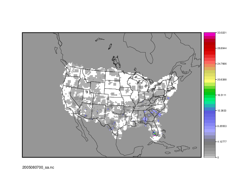
Click through the different variables to see how the performance varies over the domain. Looking at the series_cnt_RMSEvariable, are the errors larger in the south eastern or north western regions of the United States?
Why does the extent of missing data increase for CSI for the higher threshold? Compare series_cts_CSI_gt0.0 to series_cts_CSI_ge5.0. (Hint: Find the definition of Critical Success index (CSI) in the MET User's Guide and look closely at the denominator.)
Try running Plot-Data-Plane to visualize the observation rate variable for non-zero precipitation (i.e. series_fho_O_RATE_gt0.0). Since the valid range of values for this data is 0 to 1, use that to set the -plot_range option.
Setting block_size to 10000 still required 3 passes through our 185x129 grid (= 23865 grid points). What happens when you increase block_size to 24000 and re-run? Does it run slower or faster?
METplus Use Case: SeriesAnalysis
METplus Use Case: SeriesAnalysis
The SeriesAnalysis use case utilizes the MET Series-Analysis tool.
Optional: Refer to the MET Users Guide for a description of the MET tools used in this use case.
Optional: Refer to the METplus Config Glossary section of the METplus Users Guide for a reference to METplus variables used in this use case.
-
Review the use case configuration file: SeriesAnalysis.conf
This use-case shows a simple example of running Series-Analysis across precipitation forecast fields at 3 different lead times. Forecast data is from WRF output, while observational data is Stage II quantitative precipitation estimates.
Note: Forecast and observation variables are referred to individually including reference to both the NAMES and LEVELS, which relate to .
FCST_VAR1_NAME = APCP
FCST_VAR1_LEVELS = A03
OBS_VAR1_NAME = APCP_03
OBS_VAR1_LEVELS = "(*,*)"
Which relates to the following fields in the MET configuration file
field = [
{
name = "APCP";
level = [ "A03" ];
}
];
}
obs = {
field = [
{
name = "APCP_03";
level = [ "(*,*)" ];
}
];
}
Also note: Paths in SeriesAnalysis.conf may reference other config options defined in a different configuration files. For example:
where INPUT_BASE which is set in the tutorial.conf configuration file. METplus config variables can reference other config variables even if they are defined in a config file that is read afterwards.
-
Run the use case:
${METPLUS_BUILD_BASE}/parm/use_cases/met_tool_wrapper/SeriesAnalysis/SeriesAnalysis.conf \
${METPLUS_TUTORIAL_DIR}/tutorial.conf \
config.OUTPUT_BASE=${METPLUS_TUTORIAL_DIR}/output/SeriesAnalysis
METplus is finished running when control returns to your terminal console and you see the following text:
-
Review the output files:
You should have output file in the following directories:
2005080700_sa.nc
netcdf \2005080700_sa {
dimensions:
lat = 129 ;
lon = 185 ;
variables:
float lat(lat, lon) ;
lat:long_name = "latitude" ;
lat:units = "degrees_north" ;
lat:standard_name = "latitude" ;
float lon(lat, lon) ;
lon:long_name = "longitude" ;
lon:units = "degrees_east" ;
lon:standard_name = "longitude" ;
int n_series ;
n_series:long_name = "length of series" ;
float series_cnt_TOTAL(lat, lon) ;
series_cnt_TOTAL:_FillValue = -9999.f ;
series_cnt_TOTAL:name = "TOTAL" ;
series_cnt_TOTAL:long_name = "Total number of matched pairs" ;
series_cnt_TOTAL:fcst_thresh = "NA" ;
series_cnt_TOTAL:obs_thresh = "NA" ;
float series_cnt_RMSE(lat, lon) ;
series_cnt_RMSE:_FillValue = -9999.f ;
series_cnt_RMSE:name = "RMSE" ;
series_cnt_RMSE:long_name = "Root mean squared error" ;
series_cnt_RMSE:fcst_thresh = "NA" ;
series_cnt_RMSE:obs_thresh = "NA" ;
float series_cnt_FBAR(lat, lon) ;
series_cnt_FBAR:_FillValue = -9999.f ;
series_cnt_FBAR:name = "FBAR" ;
series_cnt_FBAR:long_name = "Forecast mean" ;
series_cnt_FBAR:fcst_thresh = "NA" ;
series_cnt_FBAR:obs_thresh = "NA" ;
float series_cnt_OBAR(lat, lon) ;
series_cnt_OBAR:_FillValue = -9999.f ;
series_cnt_OBAR:name = "OBAR" ;
series_cnt_OBAR:long_name = "Observation mean" ;
series_cnt_OBAR:fcst_thresh = "NA" ;
series_cnt_OBAR:obs_thresh = "NA" ;
From this output, we can see CNT line type statistics: TOTAL, RMSE, FBAR, and OBAR. These correspond to what we requested from the configuration file for output:
From the GUI that pops up, select the series_cnt_RMSE variable to view it. The image that displays is the RMSE value calculated at each grid point across the three lead times selected in the METplus configuration file.
There are two more files located in the output directory that while not statistically useful, do contain information on how METplus ran the SeriesAnalysis configuration file.
FCST_FILES contains all of the files that were found fitting the input templates for the forecast files. These are controlled by FCST_SERIES_ANALYSIS_INPUT_DIR and FCST_SERIES_ANALYSIS_INPUT_TEMPLATE. In our configuration file, these are set to
FCST_SERIES_ANALYSIS_INPUT_TEMPLATE = {init?fmt=%Y%m%d%H}/wrfprs_ruc13_{lead?fmt=%2H}.tm00_G212
Because {INPUT_BASE} is not changing for this run and the use case uses one initialization time, the lead sequences, set with the LEAD_SEQ variable and substituted in for {lead?fmt=%2H} in FCST_SERIES_ANALYSIS_INPUT_TEMPLATE, are what causes multiple files to be found. Specifically, FCST_FILES has three listed files, matching the LEAD_SEQ list from the configuration file.
Likewise, OBS_FILES contains all of the files that were found fitting the input templates for the observation files. These were controlled by OBS_SERIES_ANALYSIS_INPUT_DIR and OBS_SERIES_ANALYSIS_INPUT_TEMPLATE found in the configuration file.
-
Review the log output:
Log files for this run are found in ${METPLUS_TUTORIAL_DIR}/output/SeriesAnalysis/logs. The filename contains a timestamp of the current day.
Inside the log file all of the configuration options are listed, as well as the command that was used to call Series-Analysis:
Note that FCST_FILES and OBS_FILES were passed at runtime, rather than individual files.
There's also room for improvement noted in the low level verbosity comments of the log file:
WARNING:
WARNING: A block size of 1024 for a 185 x 129 grid requires 24 passes through the data which will be slow.
WARNING: Consider increasing "block_size" in the configuration file based on available memory.
WARNING:
This is a result of not setting the SERIES_ANALYSIS_BLOCK_SIZE in the METplus configuration file, which then defaults to the MET_INSTALL_DIR/share/met/config/SeriesAnalysisConfig_default value of 1024.
-
Create imagery for a variable in the netCDF output
While ncview was used to review the statistical imagery created by SeriesAnalysis, there is always the option to create an image using the Plot-Data-Plane tool. These images can be easily shared with others and used to demonstrate output in a presentation.
Use the following command to generate an image of the RMSE:
${METPLUS_TUTORIAL_DIR}/output/SeriesAnalysis/met_tool_wrapper/SeriesAnalysis/2005080700_sa.nc \
${METPLUS_TUTORIAL_DIR}/output/SeriesAnalysis/met_tool_wrapper/SeriesAnalysis/2005080700_RMSE.ps \
'name="series_cnt_RMSE"; level="(*,*)";'
The successful run of that command should produce an image. view it with the following command:
End of Session 3
End of Session 3
End of Session 3
Congratulations! You have completed Session 3!