Setting Up a New Experiment
Setting Up a New ExperimentSetting up a new experiment
If you choose to run a new case that is not included in the current set of DTC cases, it is relatively straightforward to do so. In order to run your own case, you will need to:
- Create necessary scripts and namelists specific to the new case
- Retrieve the data used for initial and boundary conditions (required), data assimilation (optional), and verification (optional)
There are a number of publicly available data sets that can be used for initial and boundary conditions, data assimilation, and verification. A list to get you started is available here, and we have included an automated script for downloading some forecast data from AWS, which is described on a later page. The following information will describe the necessary changes to namelists and scripts as well as provide example Docker run commands.
Creating Scripts and Namelists
Creating Scripts and NamelistsCreating Scripts and Namelists
In order to run a new case, the case-specific scripts, namelists, and other files will need to be populated under the /scripts directory. The most straightforward way to ensure you have all necessary files to run the end-to-end system is to copy a preexisting case to a new case directory and modify as needed. In this example, we will create a new case (a typical Summer weather case; spring_wx) and model the scripts after sandy_20121027:
cp -r sandy_20121027 spring_wx
cd spring_wx
At a minimum, the set_env.ksh, Vtable.GFS, namelist.wps, namelist.input, and XML files under /metviewer will need to be modified to reflect the new case. For this example, the only modifications from the sandy_20121027 case will be the date and time. Below are snippets of set_env.ksh, namelist.wps, namelist.input, and metviewer/plot_WIND_Z10.xml that have been modified to run for the spring_wx case.
set_env.ksh:
This file is used to set variables for a number of different NWP steps. You will need to change the date/time variables for your case. The comments (lines that start with the # symbol) describe each section of variables.
########################################################################
export OBS_ROOT=/data/obs_data/prepbufr
export PREPBUFR=/data/obs_data/prepbufr/2021060106/ndas.t06z.prepbufr.tm06.nr
########################################################################
# Set input format from model
export inFormat="netcdf"
export outFormat="grib2"
# Set domain lists
export domain_lists="d01"
# Set date/time information
export startdate_d01=2021060100
export fhr_d01=00
export lastfhr_d01=24
export incrementhr_d01=01
#########################################################################
export init_time=2021060100
export fhr_beg=00
export fhr_end=24
export fhr_inc=01
#########################################################################
export START_TIME=2021060100
export DOMAIN_LIST=d01
export GRID_VX=FCST
export MODEL=ARW
export ACCUM_TIME=3
export BUCKET_TIME=1
export OBTYPE=MRMS
Vtable.GFS:
On 12 June 2019, the GFS was upgraded to use the Finite-Volume Cubed-Sphere (FV3) dynamical core, which requires the use of an updated variable table from the Vtable.GFS used in the Hurricane Sandy case. The Vtable.GFS is used in running ungrib within WPS. The updated variable table for GFS data can be obtained here.
namelist.wps:
The following WPS namelist settings (in bold) will need to be changed to the appropriate values for your case. For settings with multiple values (separated by commas), only the first value needs to be changed for a single-domain WRF run:
wrf_core = 'ARW',
max_dom = 1,
start_date = '2021-06-01_00:00:00','2006-08-16_12:00:00',
end_date = '2021-06-02_00:00:00','2006-08-16_12:00:00',
interval_seconds = 10800
io_form_geogrid = 2,
/
namelist.input:
The following WRF namelist settings (in bold) will need to be changed to the appropriate values for your case. For settings with multiple values, only the first value needs to be changed for a single-domain WRF run. For the most part the values that need to be changed are related to the forecast date and length, and are relatively self-explanatory. In addition, "num_metgrid_levels" must be changed because the more recent GFS data we are using has more vertical levels than the older data:
run_days = 0,
run_hours = 24,
run_minutes = 0,
run_seconds = 0,
start_year = 2021, 2000, 2000,
start_month = 06, 01, 01,
start_day = 01, 24, 24,
start_hour = 00, 12, 12,
start_minute = 00, 00, 00,
start_second = 00, 00, 00,
end_year = 2021, 2000, 2000,
end_month = 06, 01, 01,
end_day = 02, 25, 25,
end_hour = 00, 12, 12,
end_minute = 00, 00, 00,
end_second = 00, 00, 00,
interval_seconds = 10800
input_from_file = .true.,.true.,.true.,
history_interval = 60, 60, 60,
frames_per_outfile = 1, 1000, 1000,
restart = .false.,
restart_interval = 5000,
io_form_history = 2
io_form_restart = 2
io_form_input = 2
io_form_boundary = 2
debug_level = 0
history_outname = "wrfout_d<domain>_<date>.nc"
nocolons = .true.
/
&domains
time_step = 180,
time_step_fract_num = 0,
time_step_fract_den = 1,
max_dom = 1,
e_we = 175, 112, 94,
e_sn = 100, 97, 91,
e_vert = 60, 30, 30,
p_top_requested = 1000,
num_metgrid_levels = 34,
num_metgrid_soil_levels = 4,
dx = 30000, 10000, 3333.33,
dy = 30000, 10000, 3333.33,
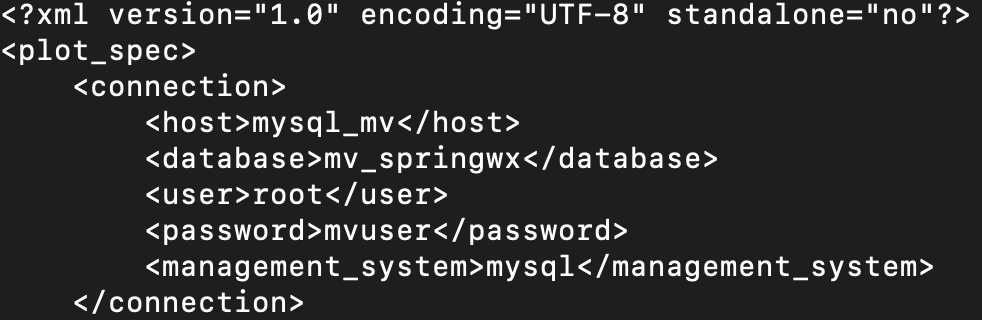
metviewer/plot_WIND_Z10.xml:
Change the database in the xml script to be "mv_springwx"
In addition, the other files can be modified based on the desired case specifics. For example, if you wish to change the variables being output in UPP, you will modify wrf_cntrl.parm (grib) or postcntrl.xml (grib2). If you are interested in changing variables, levels, or output types from MET, you will modify the MET configuration files under /met_config. More detailed information on the various components and their customization of WPS/WRF, UPP, and MET can be found in their respective User Guides:
With the scripts, namelists, and ancillary files ready for the new case, the next step is to retrieve the data for initial and boundary conditions, data assimilation, and verification.
Pulling data from AWS
Pulling data from AWSPulling data from Amazon S3 bucket
In this example, we will be retrieving 0.25° Global Forecast System (GFS) data from a publicly available Amazon Simple Storage Service (S3) bucket and storing it on our local filesystem, where it will be mounted for use in the Docker-space. The case is initialized at 00 UTC on 20210601 out to 24 hours in 3-hr increments.
To run the example case, first we need to set some variables and create directories that will be used for this specific example.
| tcsh | bash |
|---|---|
|
cd /home/ec2-user
setenv PROJ_DIR `pwd` setenv PROJ_VERSION 4.1.0
|
cd /home/ec2-user
export PROJ_DIR=`pwd` export PROJ_VERSION="4.1.0"
|
Then, you should set up the variables and directories for the experiment (spring_wx):
| tcsh | bash |
|---|---|
|
setenv CASE_DIR ${PROJ_DIR}/spring_wx
|
export CASE_DIR=${PROJ_DIR}/spring_wx
|
cd ${CASE_DIR}
mkdir -p wpsprd wrfprd gsiprd postprd pythonprd metprd metviewer/mysql
The GFS data needs to be downloaded into the appropriate directory, so we need to navigate to:
cd ${PROJ_DIR}/data/model_data/spring_wx
Next, run a script to pull GFS data for a specific initialization time (YYYYMMDDHH), maximum forecast length (HH), and increment of data (HH). For example:
If wget is not available on your system, an alternative is curl. You can, for example, modify the pull_aws_s3_gfs.ksh to have: curl -L -O
Run NWP initialization components (WPS, real.exe)
As with the provided canned cases, the first step in the NWP workflow will be to create the initial and boundary conditions for running the WRF model. This will be done using WPS and real.exe.
These commands are the same as the canned cases, with some case-specific updates to account for pointing to the appropriate scripts directory and name of the container.
SELECT THE APPROPRIATE CONTAINER INSTRUCTIONS FOR YOUR SYSTEM BELOW:
-v ${PROJ_DIR}/data/WPS_GEOG:/data/WPS_GEOG \
-v ${PROJ_DIR}/container-dtc-nwp/data:/data \
-v ${PROJ_DIR}/container-dtc-nwp/components/scripts/common:/home/scripts/common \
-v ${PROJ_DIR}/container-dtc-nwp/components/scripts/spring_wx:/home/scripts/case \
-v ${CASE_DIR}/wpsprd:/home/wpsprd \
--name run-springwx-wps dtcenter/wps_wrf:${PROJ_VERSION} /home/scripts/common/run_wps.ksh
-v ${PROJ_DIR}/data:/data \
-v ${PROJ_DIR}/container-dtc-nwp/components/scripts/common:/home/scripts/common \
-v ${PROJ_DIR}/container-dtc-nwp/components/scripts/spring_wx:/home/scripts/case \
-v ${CASE_DIR}/wpsprd:/home/wpsprd \
-v ${CASE_DIR}/wrfprd:/home/wrfprd \
--name run-springwx-real dtcenter/wps_wrf:${PROJ_VERSION} /home/scripts/common/run_real.ksh1
| tcsh | bash |
|---|---|
|
setenv TMPDIR ${CASE_DIR}/tmp
|
export TMPDIR=${CASE_DIR}/tmp
|