Graphics

This tutorial uses Python to visualize the post-processed model output. If users are familiar with Python, they may modify existing examples and/or create new plot types. As a note, while this tutorial supports plotting post-processed model output after running UPP, Python is also able to directly plot the NetCDF output from WRF (with numerous examples available online). Two customization options are provided below -- one for modifying the provided Python scripts and one for adding a new output variable to plot.

Modifying the provided Python script(s)

Users may modify existing script(s) by navigating to the /scripts/common directory and modifying the existing ALL_plot_allvars.py script (or the individual Python scripts). There are innumerable permutations for modifying the graphics scripts, based on user preferences, so one example will be chosen to show the workflow for modifying the plots. In this example, we will modify the ALL_plot_allvars.py script to change the contour levels used for plotting sea-level pressure.

Since the Hurricane Sandy case exceeds the current minimum value in the specified range, we will add 4 new contour levels. First, navigate to the Python plotting scripts directory:

Edit the ALL_plot_allvars.py script to make the desired changes to the contour levels. For this example, we will be modifying line 466 from:

To extend the plotted values starting from 960 hPa:

After the new contour levels have been added, the plots can be generated using the same run command that is used for the supplied cases. Since we are interested in the impacts on the Hurricane Sandy plots, we will use the following run command:

Adding a new plot type

In addition to modifying the ALL_plot_allvars.py for the current supported variables, users may want to add new variables to plot. The Python scripts use the pygrib module to read GRIB2 files. In order to determine what variables are available in the post-processed files and their names as used by pygrib, a simple script, read_grib.py, under the /scripts/common directory, is provided to print the variable names from the post-processed files. For this example, we will plot a new variable, wind at 850 hPa. This will require us to run the read_grib.py script to determine the required variable name. In order to run read_grib.py, we are assuming the user does not have access to Python and the necessary modules, so we will use the Python container. To enter the container, execute the following command:

Once "in" the container, navigate to the location of the read_grib.py script and open the script:

This script reads a GRIB2 file output from UPP, so this step does require that the UPP step has already been run. To execute the script:

For the standard output from the Hurricane Sandy case, here is the output from executing the script:

After perusing the output, you can see that the precipitable water variable is called 'Precipitable water.' To add the new variable to the ALL_plot_allvars.py script, it is easiest to open the script and copy the code for plotting a pre-existing variable (e.g., composite reflectivity) and modify the code for precipitable water:

In the unmodified ALL_plot_allvars.py script, copy lines 367-368 for reading in composite reflectivity, paste right below, and change the variable to be for precipitable water, where 'Precipitable water' is variable name obtained from the output of the read_grib.py: 

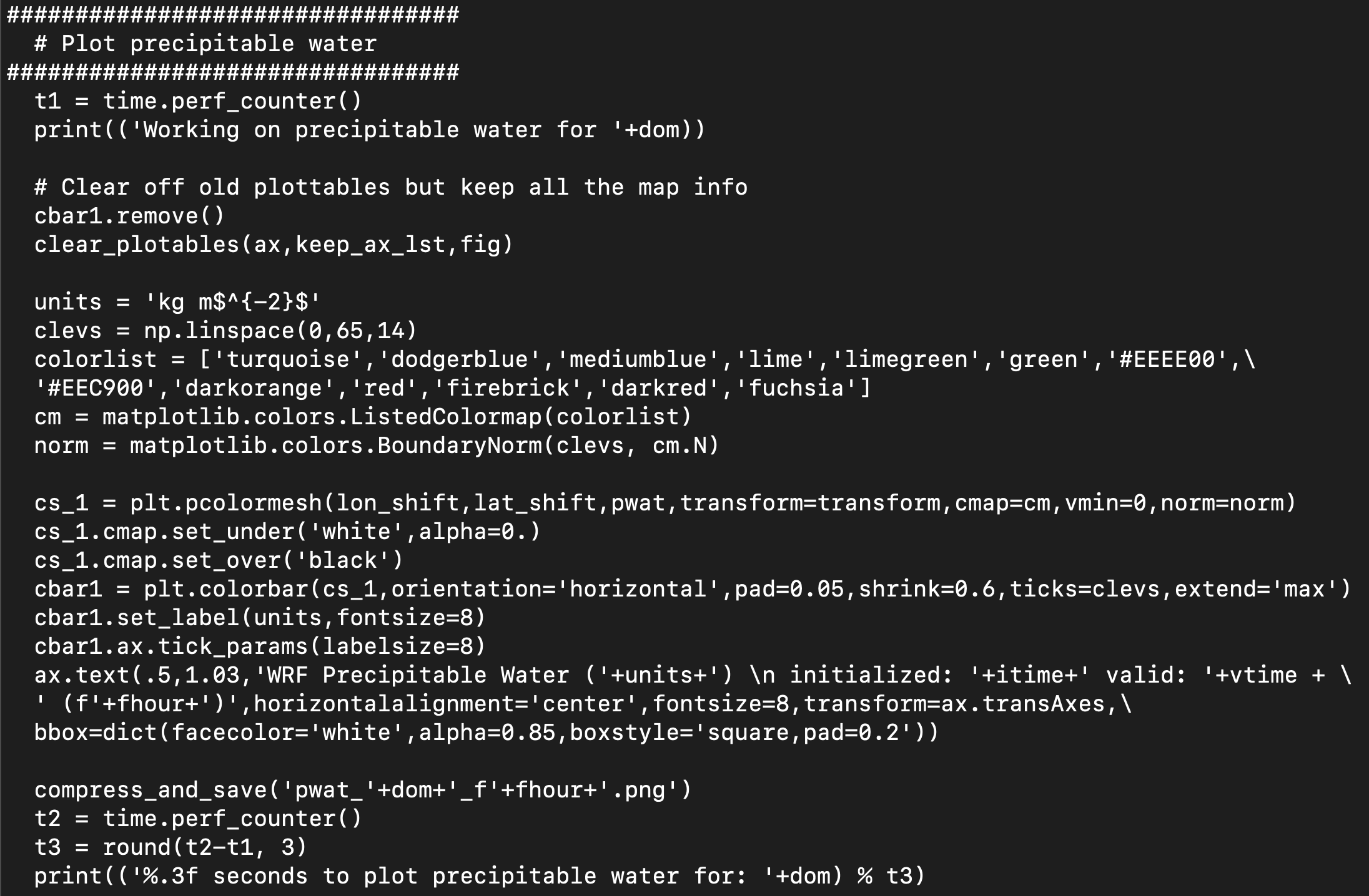
Next, we will add a new code block for plotting precipitable water, based on copying, pasting, and modifying from the composite reflectivity block above it (lines 731-760 in the unmodified code):

Note: This is a simple example of creating a new plot from the UPP output. Python has a multiple of customization options, with changes to colorbars, color maps, etc. For further customization, please refer to online resources.

To generate the new plot type, point to the scripts in the local scripts directory, run the dtcenter/python container to create graphics in docker-space and map the images into the local pythonprd directory:

After Python has been run, the plain image output files will appear in the local pythonprd directory.

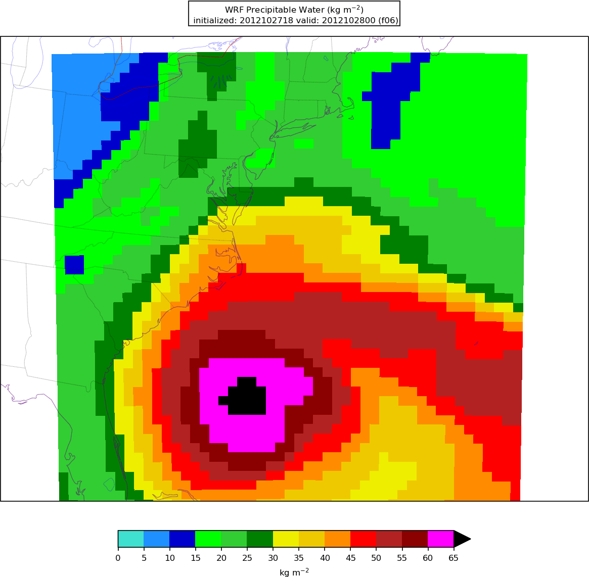
Here is an example of resulting plot of the precipitable water: