Session 2: Grid-to-Obs
Session 2: Grid-to-Obs
METplus Practical Session 2
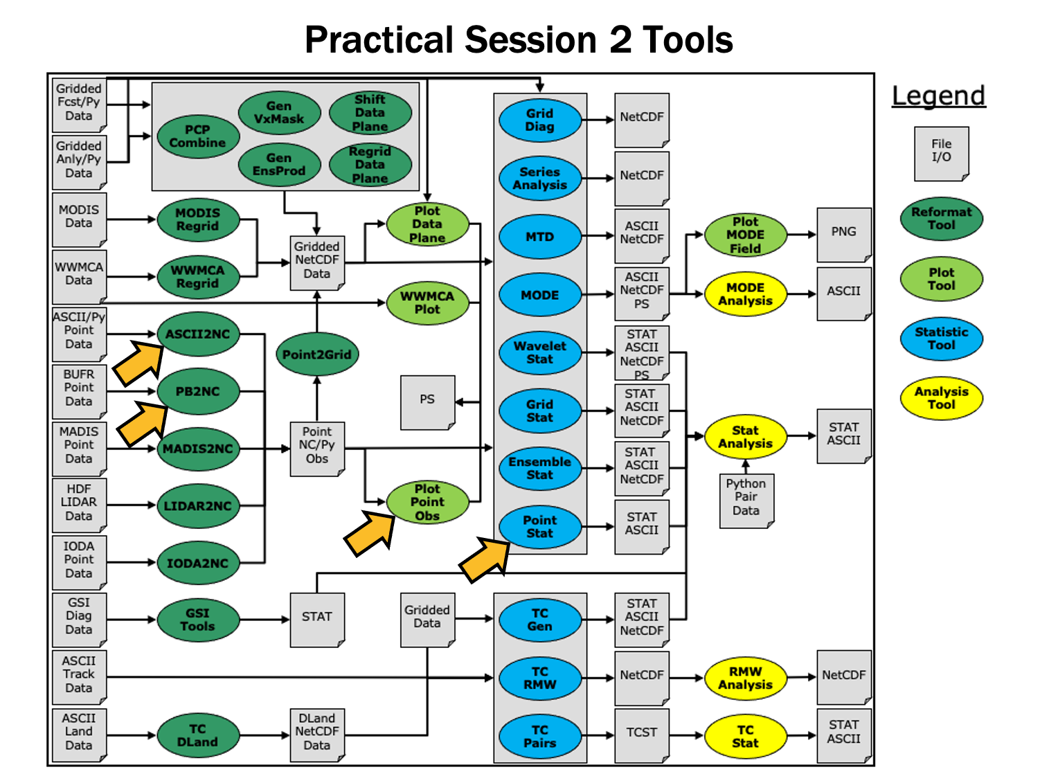
During this practical session, you will run the tools indicated below:
 You may navigate through this tutorial by following the links at the bottom of each page or by using the menu navigation.
Since you already set up your runtime environment in Session 1, you should be ready to go! To be sure, run through the following instructions to check that your environment is set correctly.
Prerequisites: Verify Environment is Set Correctly
Before running the tutorial instructions, you will need to ensure that you have a few environment variables set up correctly. If they are not set correctly, the tutorial instructions will not work properly.
EDIT AFTER COPYING and BEFORE HITTING RETURN!
source METplus-5.0.0_TutorialSetup.sh
echo ${METPLUS_BUILD_BASE}
echo ${MET_BUILD_BASE}
echo ${METPLUS_DATA}
ls ${METPLUS_TUTORIAL_DIR}
ls ${METPLUS_BUILD_BASE}
ls ${MET_BUILD_BASE}
ls ${METPLUS_DATA}
METPLUS_BUILD_BASE is the full path to the METplus installation (/path/to/METplus-X.Y)
MET_BUILD_BASE is the full path to the MET installation (/path/to/met-X.Y)
METPLUS_DATA is the location of the sample test data directory
ls ${METPLUS_BUILD_BASE}/ush/run_metplus.py
See the instructions in Session 1 for more information.
You are now ready to move on to the next section.
MET Tool: PB2NC
MET Tool: PB2NC
PB2NC Tool: General
PB2NC Functionality
The PB2NC tool is used to stratify (i.e. subset) the contents of an input PrepBufr point observation file and reformat it into NetCDF format for use by the Point-Stat or Ensemble-Stat tool. In this session, we will run PB2NC on a PrepBufr point observation file prior to running Point-Stat. Observations may be stratified by variable type, PrepBufr message type, station identifier, a masking region, elevation, report type, vertical level category, quality mark threshold, and level of PrepBufr processing. Stratification is controlled by a configuration file and discussed on the next page.
The PB2NC tool may be run on both PrepBufr and Bufr observation files. As of met-6.1, support for Bufr is limited to files containing embedded tables. Support for Bufr files using external tables will be added in a future release.
For more information about the PrepBufr format, visit:
https://emc.ncep.noaa.gov/emc/pages/infrastructure/bufrlib.php
For information on where to download PrepBufr files, visit:
https://dtcenter.org/community-code/model-evaluation-tools-met/input-data
PB2NC Usage
| Usage: pb2nc | ||
| prepbufr_file | input prepbufr path/filename | |
| netcdf_file | output netcdf path/filename | |
| config_file | configuration path/filename | |
| [-pbfile prepbufr_file] | additional input files | |
| [-valid_beg time] | Beginning of valid time window [YYYYMMDD_[HH[MMSS]]] | |
| [-valid_end time] | End of valid time window [YYYYMMDD_[HH[MMSS]]] | |
| [-nmsg n] | Number of PrepBufr messages to process | |
| [-index] | List available observation variables by message type (no output file) | |
| [-dump path] | Dump entire contents of PrepBufr file to directory | |
| [-obs_var var] | Sets the variable list to be saved from input BUFR files | |
| [-log file] | Outputs log messages to the specified file | |
| [-v level] | Level of logging | |
| [-compression level] | NetCDF file compression |
At a minimum, the input prepbufr_file, the output netcdf_file, and the configuration config_file must be passed in on the command line. Also, you may use the -pbfile command line argument to run PB2NC using multiple input PrepBufr files, likely adjacent in time.
When running PB2NC on a new dataset, users are advised to run with the -index option to list the observation variables that are present in that file.
Configure
Configure
PB2NC Tool: Configure
cd ${METPLUS_TUTORIAL_DIR}/output/met_output/pb2nc
The behavior of PB2NC is controlled by the contents of the configuration file passed to it on the command line. The default PB2NC configuration may be found in the data/config/PB2NCConfig_default file.
The configurable items for PB2NC are used to filter out the PrepBufr observations that should be retained or derived. You may find a complete description of the configurable items in the pb2nc configuration file section of the MET User's Guide or in the Configuration File Overview.
For this tutorial, edit the PB2NCConfig_tutorial_run1 file as follows:
- Set:
message_type = [ "ADPUPA", "ADPSFC" ];to retain only those 2 message types. Message types are described in:
http://www.emc.ncep.noaa.gov/mmb/data_processing/prepbufr.doc/table_1.htm - Set:
obs_window = {
beg = -1800;
end = 1800;
}so that only observations within 1800 second (30 minutes) of the file time will be retained.
- Set:
mask = {
grid = "G212";
poly = "";
}to retain only those observations residing within NCEP Grid 212, on which the forecast data resides.
- Set:
obs_bufr_var = [ "QOB", "TOB", "UOB", "VOB", "D_WIND", "D_RH" ];to retain observations for specific humidity, temperature, the u-component of wind, and the v-component of wind and to derive observation values for wind speed and relative humidity.
While we are request these observation variable names from the input file, the following corresponding strings will be written to the output file: SPFH, TMP, UGRD, VGRD, WIND, RH. This mapping of input PrepBufr variable names to output variable names is specified by the obs_prepbufr_map config file entry. This enables the new features in the current version of MET to be backward compatible with earlier versions.
Run
Run
PB2NC Tool: Run
${METPLUS_DATA}/met_test/data/sample_obs/prepbufr/ndas.t00z.prepbufr.tm12.20070401.nr \
tutorial_pb_run1.nc \
PB2NCConfig_tutorial_run1 \
-v 2
PB2NC is now filtering the observations from the PrepBufr file using the configuration settings we specified and writing the output to the NetCDF file name we chose. This should take a few minutes to run. As it runs, you should see several status messages printed to the screen to indicate progress. You may use the -v command line option to turn off (-v 0) or change the amount of log information printed to the screen.
If you'd like to filter down the observations further, you may want to narrow the time window or modify other filtering criteria. We will do that after inspecting the resultant NetCDF file.
Output
Output
PB2NC Tool: Output
When PB2NC is finished, you may view the output NetCDF file it wrote using the ncdump utility.
In the NetCDF header, you'll see that the file contains nine dimensions and nine variables. The obs_arr variable contains the actual observation values. The obs_qty variable contains the corresponding quality flags. The four header variables (hdr_typ, hdr_sid, hdr_vld, hdr_arr) contain information about the observing locations.
The obs_var, obs_unit, and obs_desc variables describe the observation variables contained in the output. The second entry of the obs_arr variable (i.e. var_id) lists the index into these array for each observation. For example, for observations of temperature, you'd see TMP in obs_var, KELVIN in obs_unit, and TEMPERATURE OBSERVATION in obs_desc. For observations of temperature in obs_arr, the second entry (var_id) would list the index of that temperature information.
Plot-Point-Obs
The plot_point_obs tool plots the location of these NetCDF point observations. Just like plot_data_plane is useful to visualize gridded data, run plot_point_obs to make sure you have point observations where you expect.
tutorial_pb_run1.nc \
tutorial_pb_run1.ps
Each red dot in the plot represents the location of at least one observation value. The plot_point_obs tool has additional command line options for filtering which observations get plotted and the area to be plotted.
By default, the points are plotted on the full globe.
tutorial_pb_run1.nc \
tutorial_pb_run1_zoom.ps \
-data_file ${METPLUS_DATA}/met_test/data/sample_fcst/2007033000/nam.t00z.awip1236.tm00.20070330.grb
MET extracts the grid information from the first record of that GRIB file and plots the points on that domain.
The plot_data_plane tool can be run on the NetCDF output of any of the MET point observation pre-processing tools (pb2nc, ascii2nc, madis2nc, and lidar2nc).
Reconfigure and Rerun
Reconfigure and Rerun
PB2NC Tool: Reconfigure and Rerun
Now we'll rerun PB2NC, but this time we'll tighten the observation acceptance criteria.
- Set:
message_type = [];to retain all message types.
- Set:
obs_window = {
beg = -25*30;
end = 25*30;
}so that only observations 25 minutes before and 25 minutes after the top of the hour are retained.
- Set:
quality_mark_thresh = 1;to retain only the observations marked "Good" by the NCEP quality control system.
${METPLUS_DATA}/met_test/data/sample_obs/prepbufr/ndas.t00z.prepbufr.tm12.20070401.nr \
tutorial_pb_run2.nc \
PB2NCConfig_tutorial_run2 \
-v 2
The majority of the observations were rejected because their valid time no longer fell inside the tighter obs_window setting.
When configuring PB2NC for your own projects, you should err on the side of keeping more data rather than less. As you'll see, the grid-to-point verification tools (Point-Stat and Ensemble-Stat) allow you to further refine which point observations are actually used in the verification. However, keeping a lot of point observations that you'll never actually use will make the data files larger and slightly slow down the verification. For example, if you're using a Global Data Assimilation (GDAS) PREPBUFR file to verify a model over Europe, it would make sense to only keep those point observations that fall within your model domain.
METplus Use Case: PB2NC
METplus Use Case: PB2NC
METplus Use Case: PB2NC
This use case utilizes the MET PB2NC tool.
Optional: Refer to the MET Users Guide for a description of the MET tools used in this use case.
Optional: Refer to the METplus Config Glossary section of the METplus Users Guide for a reference to METplus variables used in this use case.
-
Review the settings in the PB2NC.conf file:
Note that the input directory PB2NC_INPUT_DIR is set to a path relative to {INPUT_BASE} and the output directory PB2NC_OUTPUT_DIR is set to a path relative to {OUTPUT_BASE}:
...
PB2NC_INPUT_DIR = {INPUT_BASE}/met_test/data/sample_obs/prepbufr
...
PB2NC_OUTPUT_DIR = {OUTPUT_BASE}/pb2nc
{PARM_BASE} is set automatically by METplus. The wrapped MET config file for PB2NC is set relative to {PARM_BASE} in PB2NC_CONFIG_FILE:
Values for the MET tool PB2NC are passed in from METplus config files, including PB2NC.conf
//
// PB2NC configuration file.
//
// For additional information, see the MET_BASE/config/README file.
// ////////////////////////////////////////////////////////////////////////////////
//
// PrepBufr message type
//
${PB2NC_MESSAGE_TYPE} ;
//
// Mapping of message type group name to comma-separated list of values
// Derive PRMSL only for SURFACE message types
//
message_type_group_map = [
{ key = "SURFACE"; val = "ADPSFC,SFCSHP,MSONET"; },
{ key = "ANYAIR"; val = "AIRCAR,AIRCFT"; },
{ key = "ANYSFC"; val = "ADPSFC,SFCSHP,ADPUPA,PROFLR,MSONET"; },
{ key = "ONLYSF"; val = "ADPSFC,SFCSHP" }
];
No modifications are needed to run the PB2NC METplus tool.
-
Run the PB2NC use case:
${METPLUS_BUILD_BASE}/parm/use_cases/met_tool_wrapper/PB2NC/PB2NC.conf \
${METPLUS_TUTORIAL_DIR}/tutorial.conf \
config.OUTPUT_BASE=${METPLUS_TUTORIAL_DIR}/output/PB2NC
-
Review the output file:
The following is the statistical output and file generated from the command:
- sample_pb.nc
MET Tool: ASCII2NC
MET Tool: ASCII2NC
ASCII2NC Tool: General
ASCII2NC Functionality
The ASCII2NC tool reformats ASCII point observations into the intermediate NetCDF format that Point-Stat and Ensemble-Stat read. ASCII2NC simply reformats the data and does much less filtering of the observations than PB2NC does. ASCII2NC supports a simple 11-column format, described below, the Little-R format often used in data assimilation, SURFace RADiation (SURFRAD) data, Western Wind and Solar Integration Studay (WWSIS) data, and AErosol RObotic NEtwork (Aeronet) data versions 2 and 3 format. MET version 9.0 added support for passing observations to ASCII2NC using a Python script. Future version of MET may be enhanced to support additional commonly used ASCII point observation formats based on community input.
MET Point Observation Format
The MET point observation format consists of one observation value per line. Each input observation line should consist of the following 11 columns of data:
- Message_Type
- Station_ID
- Valid_Time in YYYYMMDD_HHMMSS format
- Lat in degrees North
- Lon in degrees East
- Elevation in meters above sea level
- Variable_Name for this observation (or GRIB_Code for backward compatibility)
- Level as the pressure level in hPa or accumulation interval in hours
- Height in meters above sea level or above ground level
- QC_String quality control string
- Observation_Value
It is the user's responsibility to get their ASCII point observations into this format.
ASCII2NC Usage
| Usage: ascii2nc | ||
| ascii_file1 [...] | One or more input ASCII path/filename | |
| netcdf_file | Output NetCDF path/filename | |
| [-format ASCII_format] | Set to met_point, little_r, surfrad, wwsis, aeronet, aeronetv2, aeronetv3, or python | |
| [-config file] | Configuration file to specify how observation data should be summarized | |
| [-mask_grid string] | Named grid or a gridded data file for filtering point observations spatially | |
| [-mask_poly file] | Polyline masking file for filtering point observations spatially | |
| [-mask_sid file|list] | Specific station ID's to be used in an ASCII file or comma-separted list | |
| [-log file] | Outputs log messages to the specified file | |
| [-v level] | Level of logging | |
| [-compress level] | NetCDF compression level |
At a minimum, the input ascii_file and the output netcdf_file must be passed on the command line. ASCII2NC interrogates the data to determine it's format, but the user may explicitly set it using the -format command line option. The -mask_grid, -mask_poly, and -mask_sid options can be used to filter observations spatially.
Run
Run
ASCII2NC Tool: Run
cd ${METPLUS_TUTORIAL_DIR}/output/met_output/ascii2nc
Since ASCII2NC performs a simple reformatting step, typically no configuration file is needed. However, when processing high-frequency (1 or 3-minute) SURFRAD data, a configuration file may be used to define a time window and summary metric for each station. For example, you might compute the average observation value +/- 15 minutes at the top of each hour for each station. In this example, we will not use a configuration file.
The sample ASCII observations in the MET tarball are still identified by GRIB code rather than the newer variable name option.
For example, 52 corresponds to RH:
${METPLUS_DATA}/met_test/data/sample_obs/ascii/sample_ascii_obs.txt \
tutorial_ascii.nc \
-v 2
ASCII2NC should perform this reformatting step very quickly since the sample file only contains data for 5 stations.
Output
Output
ASCII2NC Tool: Output
When ASCII2NC is finished, you may view the output NetCDF file it wrote using the ncdump utility.
The NetCDF header should look nearly identical to the output of the NetCDF output of PB2NC. You can see the list of stations for which we have data by inspecting the hdr_sid_table variable:
This ASCII data only contains observations at a few locations.
tutorial_ascii.nc \
tutorial_ascii.ps \
-data_file ${METPLUS_DATA}/met_test/data/sample_fcst/2007033000/nam.t00z.awip1236.tm00.20070330.grb \
-v 3
Next, we'll use the NetCDF output of PB2NC and ASCII2NC to perform Grid-to-Point verification using the Point-Stat tool.
METplus Use Case: ASCII2NC with Python Embedding
METplus Use Case: ASCII2NC with Python Embedding
METplus Use Case: ASCII2NC with Python Embedding
This use case utilizes the MET ASCII2NC tool to demonstrate Python Embedding. Python embedding is a novel capability within METplus that allows a user to place a Python script into a METplus workflow. For example, if a user has a data format that is unsupported by the MET tools then a user could write their own Python file reader, and hand off the data to the MET tools within a workflow.
The data utilized in this use case are hypothetical accumulated precipitation data in ASCII format.
Optional: Refer to the MET Users Guide for a description of the MET tools used in this use case.
Optional: Refer to the MET Users Guide Appendix F: Python Embedding for details on how Python embedding works for MET tools.
Optional: Refer to the METplus Config Glossary section of the METplus Users Guide for a reference to METplus variables used in this use case.
-
View the template Python Embedding scripts available with MET
MET includes example scripts for reading point data and gridded data (all in ASCII format). These can be used by users as a jumping-off point for developing their own Python embedding scripts, and are also used by this use case and other METplus use cases that demonstrate Python Embedding
met_point_obs.py
read_ascii_mpr.py
read_ascii_numpy_grid.py
read_ascii_numpy.py
read_ascii_point.py
read_ascii_xarray.py
read_met_point_obs.py
In this use case, read_ascii_point.py is used to read the sample accumulated precipitation data and serve them to ASCII2NC to format into the MET 11-column netCDF format.
-
Inspect a sample of the accumulated precipitation point data being read with Python.
These data are already in the 11-column format that MET requires, so using Python Embedding is fairly straightforward. If your data do not follow this format, some pre-processing of the data will be required to align your data to the required format. To learn more about what the 11 columns are and what MET expects each column to represent, please reference this table from the MET users guide.
-
Inspect the Python Embedding script being used in this use case
Since the sample data are point data, the Python module Pandas is utilized to read the ASCII data, assign column names that match the MET 11-column format, and then pass the data to the MET ASCII2NC tool.
-
Run the ASCII2NC Python Embedding use case:
${METPLUS_BUILD_BASE}/parm/use_cases/met_tool_wrapper/ASCII2NC/ASCII2NC_python_embedding.conf \
${METPLUS_TUTORIAL_DIR}/tutorial.conf \
config.OUTPUT_BASE=${METPLUS_TUTORIAL_DIR}/output/ASCII2NC_python_embedding
This command utilizes the METplus wrappers to execute a Python script to read in the ASCII data and pass them off to ASCII2NC to write to a netCDF file. While the Python script called here is simply for demonstration purposes, your Python script could serve to perform various data manipulation and formatting, or reading of proprietary or unsupported file formats to end up with a netCDF file compatible with the MET tools.
-
Review the Output Files
You should see the output netCDF file (ascii2nc_python.nc), which conforms to the 11-column format required by the MET tools.
-
Let's Write Some Python!
Copy the METplus use configuration file to your current working directory:
Copy the Python Embedding script to your current working directory and rename it to my_ascii_point.py:
Open the Python Embedding script in a text editor of your choice, and add the following on line 7 of the file (make sure the indentation matches the previous line):
Add on line 7:
Save the Python Embedding script.
-
Modify the METplus Use Case Configuration File to Use Your Python Script
Open the METplus use case file in a text editor of your choice and modify line 43 to use your Python script:
Change line 43 to:
The Python script contains an import of met_point_obs. This is found automatically by the read_ascii_point.py script because it is in the same share/met/python directory. Since you are calling my_ascii_point.py from your tutorial directory, you will have to set the PYTHONPATH to include the share/met/python directory so the import succeeds.
Add the following to the very end of ${METPLUS_TUTORIAL_DIR}/ASCII2NC_python_embedding.conf:
PYTHONPATH={MET_INSTALL_DIR}/share/met/python:$PYTHONPATH
Save the METplus use case configuration file.
-
Re-run the Use Case, and See If Your Python Code Is Used
${METPLUS_TUTORIAL_DIR}/ASCII2NC_python_embedding.conf \
${METPLUS_TUTORIAL_DIR}/tutorial.conf \
config.OUTPUT_BASE=${METPLUS_TUTORIAL_DIR}/output/ASCII2NC_python_embedding
-
Look for Your Python Print Statement In the METplus Log File
The 2nd last log message printed to the screen will contain the full path to the log file that was created for this run. Copy this path and run less to view the log file. It will look something like this:
(NOTE: Replace YYYYMMDDHHMMSS with the time and date appended to the log file from the run in step 8). You should see the print statement written to the log file, showing that your modifications were used by METplus and ASCII2NC!
MET Tool: Point-Stat
MET Tool: Point-Stat
Point-Stat Tool: General
Point-Stat Functionality
The Point-Stat tool provides verification statistics for comparing gridded forecasts to observation points, as opposed to gridded analyses like Grid-Stat. The Point-Stat tool matches gridded forecasts to point observation locations using one or more configurable interpolation methods. The tool then computes a configurable set of verification statistics for these matched pairs. Continuous statistics are computed over the raw matched pair values. Categorical statistics are generally calculated by applying a threshold to the forecast and observation values. Confidence intervals, which represent a measure of uncertainty, are computed for all of the verification statistics.
Point-Stat Usage
| Usage: point_stat | ||
| fcst_file | Input gridded file path/name | |
| obs_file | Input NetCDF observation file path/name | |
| config_file | Configuration file | |
| [-point_obs file] | Additional NetCDF observation files to be used (optional) | |
| [-obs_valid_beg time] | Sets the beginning of the matching time window in YYYYMMDD[_HH[MMSS]] format (optional) | |
| [-obs_valid_end time] | Sets the end of the matching time window in YYYYMMDD[_HH[MMSS]] format (optional) | |
| [-outdir path] | Overrides the default output directory (optional) | |
| [-log file] | Outputs log messages to the specified file (optional) | |
| [-v level] | Level of logging (optional) |
At a minimum, the input gridded fcst_file, the input NetCDF obs_file (output of PB2NC, ASCII2NC, MADIS2NC, and LIDAR2NC, last two not covered in these exercises), and the configuration config_file must be passed in on the command line. You may use the -point_obs command line argument to specify additional NetCDF observation files to be used.
Configure
Configure
Point-Stat Tool: Configure
cd ${METPLUS_TUTORIAL_DIR}/output/met_output/point_stat
The behavior of Point-Stat is controlled by the contents of the configuration file passed to it on the command line. The default Point-Stat configuration file may be found in the data/config/PointStatConfig_default file.
The configurable items for Point-Stat are used to specify how the verification is to be performed. The configurable items include specifications for the following:
- The forecast fields to be verified at the specified vertical levels.
- The type of point observations to be matched to the forecasts.
- The threshold values to be applied.
- The areas over which to aggregate statistics - as predefined grids, lat/lon polylines, or individual stations.
- The confidence interval methods to be used.
- The interpolation methods to be used.
- The types of verification methods to be used.
- Set:
fcst = {
message_type = [ "ADPUPA" ];
field = [
{
name = "TMP";
level = [ "P850-1050", "P500-850" ];
cat_thresh = [ <=273, >273 ];
}
];
}
obs = fcst;to verify temperature over two different pressure ranges against ADPUPA observations using the thresholds specified.
- Set:
ci_alpha = [ 0.05, 0.10 ];to compute confidence intervals using both a 5% and a 10% level of certainty.
- Set:
output_flag = {
fho = BOTH;
ctc = BOTH;
cts = STAT;
mctc = NONE;
mcts = NONE;
cnt = BOTH;
sl1l2 = STAT;
sal1l2 = NONE;
vl1l2 = NONE;
val1l2 = NONE;
pct = NONE;
pstd = NONE;
pjc = NONE;
prc = NONE;
ecnt = NONE;
eclv = BOTH;
mpr = BOTH;
}to indicate that the forecast-hit-observation (FHO) counts, contingency table counts (CTC), contingency table statistics (CTS), continuous statistics (CNT), partial sums (SL1L2), economic cost/loss value (ECLV), and the matched pair data (MPR) line types should be output. Setting SL1L2 and CTS to STAT causes those lines to only be written to the output .stat file, while setting others to BOTH causes them to be written to both the .stat file and the optional LINE_TYPE.txt file.
- Set:
output_prefix = "run1";to customize the output file names for this run.
Note that in the mask dictionary, the grid entry is set to FULL. This instructs Point-Stat to compute statistics over the entire input model domain. Setting grid to FULL has this special meaning.
Run
Run
Point-Stat Tool: Run
Next, run Point-Stat to compare a GRIB forecast to the NetCDF point observation output of the ASCII2NC tool.
${METPLUS_DATA}/met_test/data/sample_fcst/2007033000/nam.t00z.awip1236.tm00.20070330.grb \
../ascii2nc/tutorial_ascii.nc \
PointStatConfig_tutorial_run1 \
-outdir . \
-v 2
Point-Stat is now performing the verification tasks we requested in the configuration file. It should take less than a minute to run. You should see several status messages printed to the screen to indicate progress.
If you receive a syntax error such as the one listed below, review PointStatConfig_tutorial_run1 for an extra comma after the "}" on line number 59
cat_thresh = [ >273.0 ];
}, <---Remove the comma
DEBUG 1: Default Config File: /usr/local/met-9.0/share/met/config/PointStatConfig_default
DEBUG 1: User Config File: PointStatConfig_tutorial_run1
ERROR :
ERROR : yyerror() -> syntax error in file "/tmp/met_config_26760_0"
ERROR :
ERROR : line = 59
ERROR :
ERROR : column = 0
ERROR :
ERROR : text = "]"
ERROR :
ERROR :
ERROR : ];
ERROR : _____
ERROR :
Notice the more detailed information about which observations were used for each verification task. If you run Point-Stat and get fewer matched pairs than you expected, try using the -v 3 option to see why the observations were rejected.
Output
Output
Point-Stat Tool: Output
The output of Point-Stat is one or more ASCII files containing statistics summarizing the verification performed. Since we wrote output to the current directory, it should now contain 6 ASCII files that begin with the point_stat_ prefix, one each for the FHO, CTC, CNT, ECLV, and MPR types, and a sixth for the STAT file. The STAT file contains all of the output statistics while the other ASCII files contain the exact same data organized by line type.
- In the kwrite editor, select Settings->Configure Editor, de-select Dynamic Word Wrap and click OK.
- In the vi editor, type the command :set nowrap. To set this as the default behavior, run the following command:
echo "set nowrap" >> ~/.exrc
- This is a simple ASCII file consisting of several rows of data.
- Each row contains data for a single verification task.
- The FCST_LEAD, FCST_VALID_BEG, and FCST_VALID_END columns indicate the timing information of the forecast field.
- The OBS_LEAD, OBS_VALID_BEG, and OBS_VALID_END columns indicate the timing information of the observation field.
- The FCST_VAR, FCST_UNITS, FCST_LEV, OBS_VAR, OBS_UNITS, and OBS_LEV columns indicate the two parts of the forecast and observation fields set in the configure file.
- The OBTYPE column indicates the PrepBufr message type used for this verification task.
- The VX_MASK column indicates the masking region over which the statistics were accumulated.
- The INTERP_MTHD and INTERP_PNTS columns indicate the method used to interpolate the forecast data to the observation location.
- The FCST_THRESH and OBS_THRESH columns indicate the thresholds applied to FCST_VAR and OBS_VAR.
- The COV_THRESH column is not applicable here and will always have NA when using point_stat.
- The ALPHA column indicates the alpha used for confidence intervals.
- The LINE_TYPE column indicates that these are CTC contingency table count lines.
- The TOTAL column indicates the total number of matched pairs.
- The remaining columns contain the counts for the contingency table computed by applying the threshold to the forecast/observation matched pairs. The FY_OY (forecast: yes, observation: yes), FY_ON (forecast: yes, observation: no), FN_OY (forecast: no, observation: yes), and FN_ON (forecast: no, observation: no) columns indicate those counts.
- What do you notice about the structure of the contingency table counts with respect to the two thresholds used? Does this make sense?
- Does the model appear to resolve relatively cold surface temperatures?
- Based on these observations, are temperatures >273 relatively rare or common in the P850-500 range? How can this affect the ability to get a good score using contingency table statistics? What about temperatures <=273 at the surface?
- The columns prior to LINE_TYPE contain the same data as the previous file we viewed.
- The LINE_TYPE column indicates that these are CNT continuous lines.
- The remaining columns contain continuous statistics derived from the raw forecast/observation pairs. See the CNT OUTPUT FORMAT section in the Point-Stat section of the MET User's Guide for a thorough description of the output.
- Again, confidence intervals are given for each of these statistics as described above.
- What conclusions can you draw about the model's performance at each level using continuous statistics? Justify your answer. Did you use a single metric in your evaluation? Why or why not?
- Comparing the first line with an alpha value of 0.05 to the second line with an alpha value of 0.10, how does the level of confidence change the upper and lower bounds of the confidence intervals (CIs)?
- Similarly, comparing the first line with few numbers of matched pairs in the TOTAL column to the third line with more, how does the sample size affect how you interpret your results?
- The columns prior to LINE_TYPE contain the same data as the previous file we viewed.
- The LINE_TYPE column indicates that these are FHO forecast-hit-observation rate lines.
- The remaining columns are similar to the contingency table output and contain the total number of matched pairs, the forecast rate, the hit rate, and observation rate.
- The forecast, hit, and observation rates should back up your answer to the third question about the contingency table output.
- The columns prior to LINE_TYPE contain the same data as the previous file we viewed.
- The LINE_TYPE column indicates that these are MPR matched pair lines.
- The remaining columns are similar to the contingency table output and contain the total number of matched pairs, the matched pair index, the latitude, longitude, and elevation of the observation, the forecasted value, the observed value, and the climatological value (if applicable).
- There is a lot of data here and it is recommended that the MPR line_type is used only to verify the tool is working properly.
Reconfigure
Reconfigure
Point-Stat Tool: Reconfigure
Now we'll reconfigure and rerun Point-Stat.
This time, we'll use two dictionary entries to specify the forecast field in order to set different thresholds for each vertical level. Point-Stat may be configured to verify as many or as few model variables and vertical levels as you desire.
- Set:
fcst = {
field = [
{
name = "TMP";
level = [ "Z2" ];
cat_thresh = [ >273, >278, >283, >288 ];
},
{
name = "TMP";
level = [ "P750-850" ];
cat_thresh = [ >278 ];
}
];
}
obs = fcst;to verify 2-meter temperature and temperature fields between 750hPa and 850hPa, using the thresholds specified.
- Set:
message_type = ["ADPUPA","ADPSFC"];
sid_inc = [];
sid_exc = [];
obs_quality = [];
duplicate_flag = NONE;
obs_summary = NONE;
obs_perc_value = 50;to include the Upper Air (UPA) and Surface (SFC) observations in the evaluation
- Set:
mask = {
grid = [ "G212" ];
poly = [ "MET_BASE/poly/EAST.poly",
"MET_BASE/poly/WEST.poly" ];
sid = [];
llpnt = [];
}to compute statistics over the NCEP Grid 212 region and over the Eastern and Western United States, as defined by the polylines specified.
- Set:
interp = {
vld_thresh = 1.0;
shape = SQUARE;
type = [
{
method = NEAREST;
width = 1;
},
{
method = DW_MEAN;
width = 5;
}
];
}to indicate that the forecast values should be interpolated to the observation locations using the nearest neighbor method and by computing a distance-weighted average of the forecast values over the 5 by 5 box surrounding the observation location.
- Set:
output_flag = {
fho = BOTH;
ctc = BOTH;
cts = BOTH;
mctc = NONE;
mcts = NONE;
cnt = BOTH;
sl1l2 = BOTH;
sal1l2 = NONE;
vl1l2 = NONE;
val1l2 = NONE;
pct = NONE;
pstd = NONE;
pjc = NONE;
prc = NONE;
ecnt = NONE;
eclv = BOTH;
mpr = BOTH;
}to switch the SL1L2 and CTS output to BOTH and generate the optional ASCII output files for them.
- Set:
output_prefix = "run2";to customize the output file names for this run.
- 2 fields: TMP/Z2 and TMP/P750-850
- 2 observing message types: ADPUPA and ADPSFC
- 3 masking regions: G212, EAST.poly, and WEST.poly
- 2 interpolations: UW_MEAN width 1 (nearest-neighbor) and DW_MEAN width 5
Multiplying 2 * 2 * 3 * 2 = 24. So in this example, Point-Stat will accumulate matched forecast/observation pairs into 24 groups. However, some of these groups will result in 0 matched pairs being found. To each non-zero group, the specified threshold(s) will be applied to compute contingency tables.
Rerun
Rerun
Point-Stat Tool: Rerun
Next, run Point-Stat to compare a GRIB forecast to the NetCDF point observation output of the PB2NC tool, as opposed to the much smaller ASCII2NC output we used in the first run.
${METPLUS_DATA}/met_test/data/sample_fcst/2007033000/nam.t00z.awip1236.tm00.20070330.grb \
../pb2nc/tutorial_pb_run1.nc \
PointStatConfig_tutorial_run2 \
-outdir . \
-v 2
Point-Stat is now performing the verification tasks we requested in the configuration file. It should take a minute or two to run. You should see several status messages printed to the screen to indicate progress. Note the number of matched pairs found for each verification task, some of which are 0.
Plot-Data-Plane Tool
In this step, we have verified 2-meter temperature. The Plot-Data-Plane tool within MET provides a way to visualize the gridded data fields that MET can read.
${METPLUS_DATA}/met_test/data/sample_fcst/2007033000/nam.t00z.awip1236.tm00.20070330.grb \
nam.t00z.awip1236.tm00.20070330_TMPZ2.ps \
'name="TMP"; level="Z2";'
Plot-Data-Plane requires an input gridded data file, an output postscript image file name, and a configuration string defining which 2-D field is to be plotted.
-
Set the title to 2-m Temperature.
-
Set the plotting range as 250 to 305.
-
Use the color table named ${MET_BUILD_BASE}/share/met/colortables/NCL_colortables/wgne15.ctable
Next, we'll take a look at the Point-Stat output we just generated.
See the usage statement for all MET tools using the --help command line option or with no options at all.
Output
Output
Point-Stat Tool: Output
The format for the CTC, CTS, and CNT line types are the same. However, the numbers will be different as we used a different set of observations for the verification.
- The columns prior to LINE_TYPE contain header information.
- The LINE_TYPE column indicates that these are CTS lines.
- The remaining columns contain statistics derived from the threshold contingency table counts. See the point_stat output section of the MET User's Guide for a thorough description of the output.
- Confidence intervals are given for each of these statistics, computed using either one or two methods. The columns ending in _NCL(normal confidence lower) and _NCU (normal confidence upper) give lower and upper confidence limits computed using assumptions of normality. The columns ending in _BCL (bootstrap confidence lower) and _BCU (bootstrap confidence upper) give lower and upper confidence limits computed using bootstrapping.
- The columns prior to LINE_TYPE contain header information.
- The LINE_TYPE column indicates these are SL1L2 partial sums lines.
Lastly, the point_stat_run2_360000L_20070331_120000V.stat file contains all of the same data we just viewed but in a single file. The Stat-Analysis tool, which we'll use later in this tutorial, searches for the .stat output files by default but can also read the .txt output files.
METplus Use Case: PointStat
METplus Use Case: PointStat
METplus Use Case: PointStat
This use case utilizes the MET Point-Stat tool.
Optional: Refer to the MET Users Guide for a description of the MET tools used in this use case.
Optional: Refer to the METplus Config Glossary section of the METplus Users Guide for a reference to METplus variables used in this use case.
-
View Configuration File
The forecast and observations directories are specified in relation to INPUT_BASE (${METPLUS_DATA}), while the output directory is given in relation to {OUTPUT_BASE} (${METPLUS_TUTORIAL_DIR}/output).
OBS_POINT_STAT_INPUT_DIR = {INPUT_BASE}/met_test/out/pb2nc
...
POINT_STAT_OUTPUT_DIR = {OUTPUT_BASE}/point_stat
Using the PointStat configuration file, you should be able to run the use case using the sample input data set without any other changes.
-
Run the PointStat use case:
${METPLUS_BUILD_BASE}/parm/use_cases/met_tool_wrapper/PointStat/PointStat.conf \
${METPLUS_TUTORIAL_DIR}/tutorial.conf \
config.OUTPUT_BASE=${METPLUS_TUTORIAL_DIR}/output/PointStat
-
Review the output file:
The following is the statistical output and file are generated from the command:
- point_stat_360000L_20070331_120000V.stat
-
Update configuration file and re-run
vi ${METPLUS_TUTORIAL_DIR}/user_config/PointStat_tutorial.conf
BOTH_VAR1_NAME = TMP
BOTH_VAR1_LEVELS = P750-900
BOTH_VAR1_THRESH = <=273, >273
BOTH_VAR2_NAME = UGRD
BOTH_VAR2_LEVELS = Z10
BOTH_VAR2_THRESH = >=5
BOTH_VAR3_NAME = VGRD
BOTH_VAR3_LEVELS = Z10
BOTH_VAR3_THRESH = >=5
-
Rerun the use-case and compare the output
${METPLUS_TUTORIAL_DIR}/user_config/PointStat_tutorial.conf \
${METPLUS_TUTORIAL_DIR}/tutorial.conf \
config.OUTPUT_BASE=${METPLUS_TUTORIAL_DIR}/output/PointStat
${METPLUS_TUTORIAL_DIR}/output/PointStat/point_stat/point_stat_360000L_20070331_120000V.stat \
${METPLUS_TUTORIAL_DIR}/output/PointStat/point_stat/point_stat_run2_360000L_20070331_120000V.stat
METplus Use Case: PointStat - Standard Verification of Global Upper Air
METplus Use Case: PointStat - Standard Verification of Global Upper Air
METplus Use Case: PointStat - Standard Verification of Global Upper Air
This use case utilizes the MET Point-Stat tool.
Optional: Refer to the MET Users Guide for a description of the MET tools used in this use case.
Optional: Refer to the METplus Config Glossary section of the METplus Users Guide for a reference to METplus variables used in this use case.
-
View Configuration File
[statistics tool(s)]_fcst[Model]_obs[Point Data or Analysis]_[other decriptors including file format].conf
This use-case includes running two tools, PB2NC to extract the observations and then Point-Stat to compute statistics. Note the specification of wrappers to run is given in the PROCESS_LIST at the top of the file.
PROCESS_LIST = PB2NC, PointStat
BOTH_VAR1_LEVELS = P1000, P925, P850, P700, P500, P400, P300, P250, P200, P150, P100, P50, P20, P10
BOTH_VAR2_NAME = RH
BOTH_VAR2_LEVELS = P1000, P925, P850, P700, P500, P400, P300
...
BOTH_VAR5_NAME = HGT
BOTH_VAR5_LEVELS = P1000, P950, P925, P850, P700, P500, P400, P300, P250, P200, P150, P100, P50, P20, P10
Using the PointStat configuration file, you should be able to run the use case using the sample input data set without any other changes.
-
Run the PointStat use case:
${METPLUS_BUILD_BASE}/parm/use_cases/model_applications/medium_range/PointStat_fcstGFS_obsGDAS_UpperAir_MultiField_PrepBufr.conf \
${METPLUS_TUTORIAL_DIR}/tutorial.conf \
config.OUTPUT_BASE=${METPLUS_TUTORIAL_DIR}/output/PointStat_UpperAir
This may take a few minutes to run.
-
Review the output files:
If you scroll down to the middle of the file, you will notice the statistics line-type starts alternating from SL1L2 (partial_sums for continuous statistics) to VL1L2 (partial_sums for vector continuous statistics). If you scroll over, you will see that the lines are different lengths. The MET Users' Guide explains what statistics are reported in each line. See point-stat output in the MET User's Guide.
V11.0.0 gfs NA 000000 20170601_000000 20170601_000000 000000 20170531_231500 20170601_004500 UGRD_VGRD m/s P1000 UGRD_VGRD NA P1000 ADPUPA FULL BILIN 4 NA NA NA NA VL1L2 274 -0.94226 0.58128 -0.73759 0.71095 28.62333 34.35785 32.59062 4.94574 4.67908
V11.0.0 gfs NA 000000 20170601_000000 20170601_000000 000000 20170531_231500 20170601_004500 VGRD m/s P925 VGRD NA P925 ADPUPA FULL BILIN 4 NA NA NA NA SL1L2 523 0.45376 0.44876 29.18591 29.53347 32.41237 1.34806
V11.0.0 gfs NA 000000 20170601_000000 20170601_000000 000000 20170531_231500 20170601_004500 UGRD_VGRD m/s P925 UGRD_VGRD NA P925 ADPUPA FULL BILIN 4 NA NA NA NA VL1L2 523 0.67347 0.45376 0.81969 0.44876 67.86401 67.37296 74.9574 6.98307 7.34872
-
Update configuration file and re-run
Let's look at the two line-types separately in a more human-readable format.
POINT_STAT_OUTPUT_FLAG_VL1L2 = BOTH
-
Rerun the use-case and compare the output
${METPLUS_TUTORIAL_DIR}/user_config/PointStat_UpperAir_example2.conf \
${METPLUS_TUTORIAL_DIR}/tutorial.conf \
config.OUTPUT_BASE=${METPLUS_TUTORIAL_DIR}/output/PointStat_UpperAir_example2
point_stat_000000L_20170601_000000V.stat
point_stat_000000L_20170601_000000V_vl1l2.txt
point_stat_000000L_20170602_000000V_sl1l2.txt
point_stat_000000L_20170602_000000V.stat
point_stat_000000L_20170602_000000V_vl1l2.txt
point_stat_000000L_20170603_000000V_sl1l2.txt
point_stat_000000L_20170603_000000V.stat
point_stat_000000L_20170603_000000V_vl1l2.txt
Inspect the .txt files, they should have the same data as in the .stat file, just separated by line type. You will notice the header includes the name of statistics in the .txt files because they are specific to each line type.
METplus Use Case: PointStat - Standard Verification for CONUS Surface
METplus Use Case: PointStat - Standard Verification for CONUS Surface
METplus Use Case: PointStat - Standard Verification of CONUS Surface
This use case utilizes the MET Point-Stat tool.
Optional: Refer to the MET Users Guide for a description of the MET tools used in this use case.
Optional: Refer to the METplus Config Glossary section of the METplus Users Guide for a reference to METplus variables used in this use case.
-
View Configuration File
Many of the options are similar, except the fields typically at the surface (BOTH_VARn_LEVELS = Z2 and Z10 or integrated BOTH_VARn_LEVELS = L0). Also, the Point-Stat MESSAGE_TYPE is set to a specific keyword ONLYSF for only surface fields. Finally, the PB2NC_INPUT_TEMPLATE includes a da_init specification in the input template to help determine the valid time of the data.
...
PB2NC_INPUT_TEMPLATE = nam.{da_init?fmt=%Y%m%d}/nam.t{da_init?fmt=%2H}z.prepbufr.tm{offset?fmt=%2H}
Using this configuration file, you should be able to run the use case using the sample input data set without any other changes.
-
Run the PointStat use case
${METPLUS_BUILD_BASE}/parm/use_cases/model_applications/medium_range/PointStat_fcstGFS_obsNAM_Sfc_MultiField_PrepBufr.conf \
${METPLUS_TUTORIAL_DIR}/tutorial.conf \
config.OUTPUT_BASE=${METPLUS_TUTORIAL_DIR}/output/PointStat_Sfc
This may take a few minutes to run.
-
Review the output files
Inspection of the file shows that statistics for TMP, RH, UGRD, VGRD, UGRD_VGRD are available. Also, based on the number listed after the line type (SL1L2 and VL1L2), there are between 8263 - 9300 points included in the computation of the statistics. The big question is why are there no statistics for TCDC and PRMSL? Let's look at the log files.
Open the log file and search on TCDC, you will see that there is an error message stating "no fields matching TCDC/L0 found" in the GFS file. That is why TCDC does not appear in the output.
Look for PRMSL/Z0 in the log file. We can see the following:
DEBUG 2: Number of matched pairs = 0
DEBUG 2: Observations processed = 441178
DEBUG 2: Rejected: station id = 0
DEBUG 2: Rejected: obs var name = 441178
You will note, the number of observations processed is the same as the number rejected due to a mismatch with the obs var name. That suggests we need to look at how the OBS variable for PRMSL is defined.
-
Inspect configuration file and plot fields
Note that PB2NC_OBS_BUFR_VAR_LIST = PMO, TOB, TDO, UOB, VOB, PWO, TOCC, D_RH, where PMO is the identifier for MEAN SEA-LEVEL PRESSURE OBSERVATION according to https://www.nco.ncep.noaa.gov/sib/decoders/BUFRLIB/toc/prepbufr/prepbufr_bftab/. Let's use Plot-Data-Plane to confirm this identifier will provide valid observations for Point-Stat to use.
${METPLUS_TUTORIAL_DIR}/output/PointStat_Sfc/nam/conus_sfc/20170601/nam.2017060100.nc \
${METPLUS_TUTORIAL_DIR}/output/PointStat_Sfc/nam/conus_sfc/20170601/nam.2017060100.ps \
-obs_var PMO
${METPLUS_TUTORIAL_DIR}/output/PointStat_Sfc/nam/conus_sfc/20170601/nam.2017060100.ps \
${METPLUS_TUTORIAL_DIR}/output/PointStat_Sfc/nam/conus_sfc/20170601/nam.2017060100.png
display ${METPLUS_TUTORIAL_DIR}/output/PointStat_Sfc/nam/conus_sfc/20170601/nam.2017060100.png
-
Update configuration file and re-run
FCST_VAR7_LEVELS = Z0
OBS_VAR7_NAME = PMO
OBS_VAR7_LEVELS = Z0
${METPLUS_TUTORIAL_DIR}/user_config/PointStat_Sfc2.conf \
${METPLUS_TUTORIAL_DIR}/tutorial.conf \
config.OUTPUT_BASE=${METPLUS_TUTORIAL_DIR}/output/PointStat_Sfc2
There is now a line with PRMSL listed and statistics reported.
End of Session 2 and Additional Exercises
End of Session 2 and Additional Exercises
End of Session 2
Congratulations! You have completed Session 2!
If you have extra time, you may want to try this additional METplus exercise.
The default statistics created by this exercise only dump the partial sums, so we will be also modifying the MET configuration file to add the continuous statistics to the output. There is a little more setup in this use case, which will be instructive and demonstrate the basic structure, flexibility and setup of METplus configuration.
${METPLUS_TUTORIAL_DIR}/user_config/PointStat_add_linetype.conf
to
to
${METPLUS_TUTORIAL_DIR}/user_config/PointStat_add_linetype.conf \
${METPLUS_TUTORIAL_DIR}/tutorial.conf \
config.OUTPUT_BASE=${METPLUS_TUTORIAL_DIR}/output/PointStat_AddLinetype
point_stat_360000L_20070331_120000V.stat
point_stat_360000L_20070331_120000V_vcnt.txt