Case 6: Cycling Case
Case 6: Cycling Case
GSI CYCLING RUN ARW BACKGROUND
Introduction
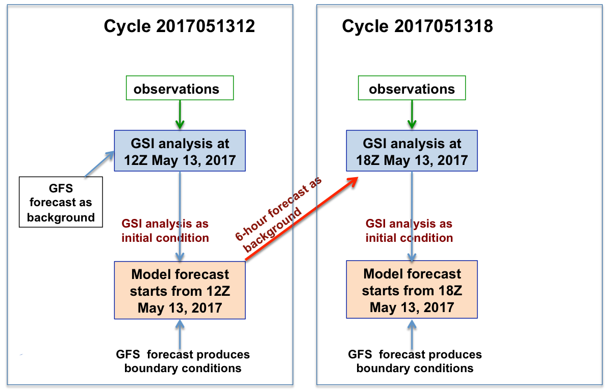
This exercise illustrate the basic structure and flow of a cycling data assimilation system, as shown in this chart (time doesn't match with the new case). It consists of running the GSI analysis with an ARW netcdf background field, and then the GSI analysis provides the initial fields for running a WRF-ARW forecast. The forecast output can be used as the GSI background for next GSI analysis.
The regional NAM BE is employed as the background error covariance and only conventional observations are assimilated in this example.
There are 4 steps in this GSI-ARW cycling data assimilation exercise:
- Step 1: GSI Data Analysis for 12Z of August 12, 2018. This step is similar to the online exercise ARW 3DVAR with conventional data (PrepBUFR)
- Step 2: WRF-ARW model forecast at 12Z of August 12, 2018, using the GSI analysis from step 1.
- Step 3: GSI Data Analysis for 18Z of August 12, 2018, using the 6-hour forecast output from step 2.
- Step 4: WRF-ARW model forecast at 18Z of August 12, 2018, using the GSI analysis from step 3.
GSI analysis at 12Z
GSI analysis at 12Z
GSI CYCLING RUN ARW BACKGROUND
GSI analysis at 12Z
For this step of GSI analysis at 12Z of August 12, 2018, we will use the GSI analysis output
wrf_inoutfrom the online exercise 03 ARW 3DVAR with conventional data (PrepBUFR) .
If you haven't practiced case 03, simply follow the steps in the above link to perform the GSI data assimilation and get the analysis.
Set up WRF-ARW run at 12Z
Set up WRF-ARW run at 12Z
GSI CYCLING RUN ARW BACKGROUND
Set up WRF-ARW run at 12Z
For this step of WRF-ARW run at 12Z of August 12, 2018, we will use the GSI analysis output
wrf_inoutfrom the online exercise 05 as the initial fields to launch 6-hour WRF forecast.
First, make sure you have a compiled code of the latest WRF-ARW code (V4.0). You can download the boundary condition for WRF from link .
Please follow the WRF tutorial and documents for the details of the WRF system application.
Here we provide the namelist file for reference of WRF run:
namelist.input
Running the ARW and checking the forecast results
The ARW can be run by creating a run script run_wrf.ksh and submitting it in the run directory:
bsub < run_wrf.kshIt will take a few minutes to finish. Once done, users should see the forecast files in each forecast hour from 12z to 20z like
wrfout_d01_2018-08-12_HH_00:00:00.The contents of this run directory are provided in the following list .
The ARW standard output file rsl.out.0000 is povided for reference.
GSI analysis at 18Z
GSI analysis at 18Z
GSI CYCLING RUN ARW BACKGROUND
GSI analysis at 18Z
For this step of GSI analysis at 18Z of August 12, 2018, we will use the 6-hour forecast output from the WRF run at 12Z as the background and conventional observations at 18Z. The steps to set up the GSI analysis is very similar to case 03, except for the background field and observations. The example run script can be found here.
Running the GSI run Script and checking the results
After GSI runs, a run directory will be created according to the path set in the variable
WORK_ROOT. The contents of this run directory are provided in the following list .The standard output file
stdoutand the fit files for this GSI run: temperature (fit_t1); wind (fit_w1); moisture (fit_q1).Convergence information (section 4.6 of the GSI User's Guide) is available in the file: fort.220
WRF-ARW run at 18Z
As a continued data assimilation run, the 18Z GSI analysis from the above step is then used as the initial field, together with the WRF background conditions at 18Z, to launch the WRF forecast at 18Z. The steps are very similar to the WRF run at 12Z and therefore not repeated here.