Session 1: METplus Setup/Grid-to-Grid
Session 1: METplus Setup/Grid-to-Grid
METplus Practical Session 1
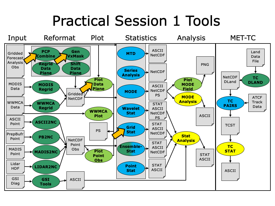
During the first METplus practical session, you will run the tools indicated below:
During this practical session, please work on the Session 1 exercises. Proceed through the tutorial exercises by following the navigation links at the bottom of each page.
Each practical session builds on the output of previous practical sessions. So please work on them in the order listed.
Throughout this tutorial, code blocks in BOLD white text with a black background should be copied from your browser and pasted on the command line. You can copy-and-paste the text using one of two methods:
- Use the mouse:
- Hold down the left mouse button to select the text
- Place the mouse in the desired location and click the middle mouse button once to paste the selected text
- Use the Copy and Paste options:
- Hold down the left mouse button to select the text
- Click the right mouse button and select the option for Copy
- Place the mouse in the desired location, click the right mouse button, and select the option for Paste
Note: Instructions in this tutorial use vi to open and edit files. If you prefer to use a different file editor, feel free to substitute it whenever you see vi.
Note: Instructions in this tutorial use okular to view pdf, ps, and png files. If you prefer to use a different file viewer, feel free to substitute it whenever you see okular.
Click the 'METplus Setup >' on the bottom right to get started!
METplus Setup
METplus Setup
METplus Overview
METplus is a set of python modules that have been developed with the flexibility to run MET for various use cases or scenarios. The goal is to simplify the running of MET for scientists. Currently, the primary means of achieving this is through the use of METplus configuration files, aka. "conf files". It is designed to provide a framework in which additional MET use cases can be added. The conf file implementation utilizes a Python package called produtil that was developed by NOAA/NCEP/EMC for the HWRF system.
The METplus Python application is designed to be run as stand alone module files - calling one MET process; through a user defined process list - as in this tutorial; or within a workflow management system on an HPC cluster - which is TBD.
Please be sure to follow the instructions in order.
METplus Useful Links
The following links are just for reference, and not required for this practical session. A METplus release is available on GitHub, and provides sample data and instructions.
GitHub METplus links
The METplus-related code repositories are available in GitHub in the following locations:
- https://github.com/NCAR/METplus - Python wrappers and use cases
- https://github.com/NCAR/MET - Core MET codebase
- https://github.com/NCAR/METviewer - Display system for MET output
- https://github.com/NCAR/METdb - Database system for MET output (currently private)
- https://github.com/NCAR/METplotpy - Python plotting scripts (currently private)
- https://github.com/NCAR/METcalcpy - Python calculation functions (currently private)
- METexpress - Streamlined display system (currently lives in NOAA's VLab)
New features are developed and bugs are tracked using GitHub issues in each repository.
METplus: Initial setup
METplus: Initial setup
Prequisites: Software
The following is a full list of software that is required to utilize all the functionality in METplus.
NOTE: We will not by running the cyclone plotter or grid plotting scripts in this tutorial. So the additional libraries mentioned below are not installed.
- Python 2.7.x
- Additional Python libraries: - required by the cyclone plotter and grid plotting scripts.
- numpy
- matplotlib - not installed, Is is not required for this tutorial.
- cartopy - not installed, It is not required for this tutorial.
- MET 8.1 - already installed locally on the tutorial machines.
- R - used by TCMPRPlotter wrapper, Wraps the MET plot_tcmpr.R script
- ncap2 - NCO netCDF Operators
- wgrib2 - only needed for series analysis wrappers (SeriesByLead and SeriesByInit)
- ncdump - NetCDF binaries
- convert - Utilitity from ImageMagick software suite
Prequisites: Environment
Before running these instructions, you will need to ensure that you have a few environment variables set up correctly. If they are not set correctly, these instructions will not work properly.
- Check that you have METPLUS_TUTORIAL_DIR set correctly:
If you don't see a path in your user directory output to the screen, set this environment variable in your user profile before continuing.
- Check that you have METPLUS_BUILD_BASE, MET_BUILD_BASE, and METPLUS_DATA set correctly:
echo ${MET_BUILD_BASE}
echo ${METPLUS_DATA}
If any of these variables are not set, please set them. They will be referenced throughout the tutorial.
MET_BUILD_BASE is the full path to the MET installation (/path/to/met-X.Y)
METPLUS_DATA is the location of the sample test data directory
- Check that you have loaded the MET module correctly:
You should see the usage statement for Point-Stat. The version number listed should correspond to the version listed in MET_BUILD_BASE. If it does not, you will need to either reload the met module, or add ${MET_BUILD_BASE}/bin to your PATH.
Getting The Software
For this tutorial we'll use the METplus v2.2 release, which has been installed in a common location. We will configure METplus to run the met-8.1 software, which has also been installed in a common location. We will copy the parameter files from the shared METplus location to your own directory so you can modify them without changing the shared installation settings.
Please use the following instructions to setup METplus on your tutorial machine:
- Create a directory to store your METplus files (include the version number for traceability):
- Create a symbolic link so that you can refer to the METplus directory instead of METplus-2.2 (you may need to remove the link if it already exists):
ln -s METplus-2.2 METplus
- List the contents of the metplus_tutorial directory:
You should see something similar to this:
drwxrwxr-x 2 mccabe rap 4096 Jul 18 15:34 METplus-2.2
- Copy the parm directory from the shared METplus location to your home directory:
- Create directory to store configuration files you will create:
For reference, the following are instructions to download and install METplus on your own machine.
- If you wish, download and unpack the release tarball and create a METplus symbolic link:
DO NOT RUN THESE COMMANDS FOR THE TUTORIAL!
wget https://github.com/NCAR/METplus/archive/v2.2.tar.gz
tar -xvzf METplus_v2.2.tar.gz
rm METplus
ln -s METplus-2.2 METplus
Sample Data Input and Location of Output
The Sample Input Data used to run the examples in this tutorial already exist in a shared location. For reference, here are example instructions to obtain the sample input data.
DO NOT RUN THESE COMMANDS FOR THE TUTORIAL!
cd /d1/METplus-2.2_Data
wget https://github.com/NCAR/METplus/releases/download/v2.2/sample_data-grid_to_grid-2.2.tgz
tar -xvzf sample_data-grid_to_grid-2.2.tgz
rm sample_data-grid_to_grid-2.2.tgz
This will create a directory named 'grid_to_grid' under '/d1/METplus_Data' that contains all of the sample input data needed to run the grid_to_grid use cases (found in parm/use_cases/grid_to_grid/examples). Other sample data tarballs are available under 'Assets' on the METplus GitHub releases page.
When running METplus wrapper use cases, all output is placed in the ${METPLUS_TUTORIAL_DIR}/output directory.
When running MET on the command line, all output will be written to ${METPLUS_TUTORIAL_DIR}/output/met_output
Your Runtime Environment
For this tutorial, the MET software is available via a module file. This has already been loaded for all users, so the MET software is available when you login.
The PATH environment variable is set to allow the METplus scripts to be run from any directory.
- Edit the .bash_profile file to configure your runtime environment for use with METplus:
Add the following at the end of the file to set the PATH and METPLUS_PARM_BASE environment variables. Also update LD_LIBRARY_PATH to avoid runtime NetCDF linker errors:
bash:
export METPLUS_PARM_BASE=${METPLUS_TUTORIAL_DIR}/METplus/parm
export LD_LIBRARY_PATH=/software/depot/met-8.1/external_libs/lib:${LD_LIBRARY_PATH}
csh:
setenv METPLUS_PARM_BASE ${METPLUS_TUTORIAL_DIR}/METplus/parm
setenv LD_LIBRARY_PATH /software/depot/met-8.1/external_libs/lib:${LD_LIBRARY_PATH}
Save and close that file, then source it to apply the settings to the current shell. The next time you login, you do not have to source this file again:
If you did everything correctly, running 'which master_metplus.py' should show you the path to the script in the shared location, ${METPLUS_BUILD_BASE}:
METplus: Directories and Configuration Files - Overview
METplus: Directories and Configuration Files - Overview
METplus directory structure
Brief description and overview of the METplus/ directory structure.
- doc/ - Doxygen files for building the html API documentation.
- doc/METplus_Users_Guide - LyX files and the user guide PDF file.
- internal_tests/ - for engineering tests
- parm/ - where config files live
- README.md - general README
- sorc/ - executables and documentation build system
- ush/ - python scripts
METplus default configuration files
The METplus default configuration files metplus_system.conf, metplus_data.conf, metplus_runtime.conf, and metplus_logging.conf are always read by default and in the order shown. Any additional configuration files passed in on the command line are than processed in the order in which they are specified. This allows for each successive conf file the ability to override variables defined in any previously processed conf files. It also allows for defining and setting up conf files from a general (settings used by all use cases, ie. MET install dir) to more specific (Plot type when running track and intensity plotter) structure. The idea is to created a hiearchy of conf files that is easier to maintain, read, and manage. It is important to note, running METplus creates a single configuration file, which can be viewed to understand the result of all the conf file processing.
The final metplus conf file is defined here:
metplus_runtime.conf:METPLUS_CONF={OUTPUT_BASE}/metplus_final.conf
Use this file to see the result of all the conf file processing, this can be very helpful when troubleshooting,
NOTE: The syntax for METplus configuration files MUST include a "[section]" header with the variable names and values on subsequent lines.
Unless otherwise indicated, all directories are relative to your ${METPLUS_PARM_BASE} directory.
The metplus_config directory - there are four config files:
- metplus_system.conf
- contains "[dir]" and "[exe]" to set directory and executable paths
- any information specific to host machine
- metplus_data.conf
- Sample data or Model input location
- filename templates and regex for filenames
- metplus_runtime.conf
- contains "[config]" section
- var lists, stat lists, configurations, process list
- anything else needed at runtime
- metplus_logging.conf
- contains "[dir]" section for setting the location of log files.
- contains "[config]" section for setting various logging configuration options.
The use_cases directory - The use cases:
This is where the use cases you will be running exist. The use case filenaming and directory structure is by convention. It is intended to simplify management of common configuration items for a specific use case. Under the use_cases directory is a subdirectory for each use case. Under that is an examples subdirectory and a more general configuration file that contains information that is shared by examples of the use case.
- For example, the track and intensity use case conf directory and file structure.
- track_and_intensity - directory
- track_and_intensity/track_and_intensity.conf - use case configuration file
- track_and_intensity/examples - directory to hold various track and intensity example conf files.
- track_and_intensity/examples/tcmpr_mean_median.conf - specific use case
- track_and_intensity/examples/README - File containing instructions to run the use case examples in this directory.
Within each use case there is a met_config subdirectory that contains MET specific config files for that use case. The use_cases/<use case>/met_config directory - store all your MET config files, e.g.:
- GridStatConfig_anom (for MET grid_stat)
- TCPairsETCConfig (for MET tc_pairs)
- SeriesAnalysisConfig_by_init (for MET series_analysis)
- SeriesAnalysisConfig_by_lead (for MET series_analysis)
METplus: User Configuration Settings
METplus: User Configuration Settings
Modify your METplus conf files
In this section you will modify the configuration files that will be read for each call to METplus.
The paths in this practical assume:
- You have copied the parm directory from the shared METplus location into your ${METPLUS_TUTORIAL_DIR}/METplus directory
- You have added the shared METplus ush directory to your PATH
- You have set the METPLUS_PARM_BASE environment variable to your copied parm directory
- You are using the shared installation of MET.
If not, then you need to adjust accordingly.
- Try running master_metplus.py. You should see the usage statement output to the screen.
- Now try to pass in the example.conf configuration file found in your parm directory under use_cases/wrappers/examples
You should see an error message stating that OUTPUT_BASE was not set correctly. You will need to configure the METplus wrappers to be able to run a use case.
The values in the default metplus_system.conf, metplus_data.conf, metplus_runtime.conf, and metplus_logging.conf configuration files are read in first when you run master_metplus.py. The settings in these files can be overridden in the use case conf files and/or a user's custom configuration file.
Some variables in the system conf are set to '/path/to' and must be overridden to run METplus, such as OUTPUT_BASE in metplus_system.conf.
- View the metplus_system.conf file and notice how OUTPUT_BASE = /path/to . This implies it is REQUIRED to be overridden to a valid path.
Note: The default installation of METplus has /path/to values for MET_INSTALL_DIR, TMP_DIR, and INPUT_BASE. These values were set in the shared METplus configuration when it was installed. This was done because these settings will likely be set to the same values for all users.
- Change directory to your ${METPLUS_PARM_BASE} directory and modify the METplus base configuration files using the editor of your choice (vi listed as an example).
If METPLUS_PARM_BASE is set correctly, you should now be in ${METPLUS_TUTORIAL_DIR}/METplus/parm/metplus_config
Note: A METplus conf file is not a shell script.
You CAN NOT refer to environment variables as you would in a shell script or command prompt, i.e. ${HOME}.
Instead, you must reference the environment variable $HOME as {ENV[HOME]}
Reminder: Make certain to maintain the KEY = VALUE pairs under their respective current [sections] in the conf file.
- Set the [dir] INPUT_BASE variable to the location of the METplus sample data that will be used in the exercises
- Set the [dir] OUTPUT_BASE variable to the location you will write output data
Set the [dir] MET_INSTALL_DIR variable to the location where MET is installed (this should already be done when METplus was installed in the shared location)
Set the [dir] TMP_DIR variable to a location you have write permissions
MET_INSTALL_DIR = {ENV[MET_BUILD_BASE]}
TMP_DIR = {OUTPUT_BASE}/tmp
NOTE: When installing METplus, you will need to set the full path to the non-MET executables in the metplus_system.conf file if they are not found in the user's path. This step was completed when METplus was installed in the shared location.
Creating user conf files
You can create additional configuration files to be read by the METplus wrappers to override variables.
Reminder: When adding variables to be overridden, make sure to place the variable under the appropriate section.
For example, [config], [dir], [exe]. If necessary, refer to the default appropriate parm/metplus_config conf files to determine the [section] that corresponds to the variable you are overriding. The value set will be the last one in the sequence of configuration files. See OUTPUT_BASE/metpus_final.conf to see what values were used for a given METplus run.
- Create a new configuration file in your user_config directory and override the [dir] OUTPUT_BASE variable to point to a different location.
vi change_output_base.conf
Copy and paste the following text into the file and save it.
OUTPUT_BASE = {ENV[METPLUS_TUTORIAL_DIR]}/output_changed
We will test out using these configurations on the next page.
METplus: How to Run
METplus: How to Run
Running METplus
Running METplus involves invoking the python script master_metplus.py followed by a list of configuration files using the -c option for each additional conf file.
Reminder: The default set of conf files are always read in and processed in the following order;
metplus_system.conf, metplus_data.conf, metplus_runtime.conf, metplus_logging.conf.
If you have configured METplus correctly and run master_metplus.py without passing in any configuration files, it will generate a usage statement to indicate that other config files are required to perform a useful task. It will generate an error statement if something is amiss.
- Review the example.conf configuration file
- Call the master_metplus.py script, passing in the example.conf configuration file with the -c command line option. You should see logs output to the screen.
Note: If master_metplus.py can't be found, you may need to add it to the path. Optionally, you can specify the full path to the script.
Note: The environment variable METPLUS_PARM_BASE determines where to look for relative paths to configuration files. If the environment variable is not set, the script will look in the parm directory that is associated with the version of master_metplus.py that is being called. Optionally, you can specify the full path to the configuration files.
OPTIONAL:
- Check the directory specified by the OUTPUT_BASE configuration variable. You should see that files and sub-directories have been created
- Review the master log file to see what was run. Compare the log output to the example.conf configuration file to see how they correspond to each other. The log file will have today's date in the filename
You will notice that METplus ran for 4 valid times, processing 4 forecast hours for each valid time. For each run, it used the input template to determine which file to look for.
- Now run METplus passing in the example.conf from the previous run AND your newly created configuration file.
- Check the directory specified by the OUTPUT_BASE configuration variable that you set in the change_output_base.conf configuration file. You should see that files and sub-directories have been created in the new location.
Remember: Additional conf files are processed after the metplus_config files in the order specified on the command line.
Order matters, since each successive conf file will override any variable defined in a previous conf file.
Note: The processing order allows for structuring your conf files from general (variables shared-by-all) to specific (variables shared-by-few).
MET Tool: PCP-Combine
MET Tool: PCP-Combine
We now shift to a dicussion of the MET PCP-Combine tool and will practice running it directly on the command line. Later in this session, we will run PCP-Combine as part of a METplus use case.
PCP-Combine Functionality
The PCP-Combine tool is used (if needed) to add, subtract, or sum accumulated precipitation from several gridded data files into a single NetCDF file containing the desired accumulation period. It's NetCDF output may be used as input to the MET statistics tools. PCP-Combine may be configured to combine any gridded data field you'd like. However, all gridded data files being combined must have already been placed on a common grid. The copygb utility is recommended for re-gridding GRIB files. In addition, the PCP-Combine tool will only sum model files with the same initialization time unless it is configured to ignore the initialization time.
PCP-Combine Usage
View the usage statement for PCP-Combine by simply typing the following:
| Usage: pcp_combine | ||
| [[-sum] sum_args] | [-add input_files] | [-subtract input_files] | [-derive stat_list input_files] (Note: "|" means "or") |
||
| [-sum] sum_args | Precipitation from multiple files containing the same accumulation interval should be summed up using the arguments provided. | |
| -add input_files | Data from one or more files should be added together where the accumulation interval is specified separately for each input file. | |
| -subtract input_files | Data from exactly two files should be subtracted. | |
| -derive stat_list input_files | The comma-separated list of statistics in "stat_list" (sum, min, max, range, mean, stdev, vld_count) should be derived using data from one or more files. | |
| out_file | Output NetCDF file to be written. | |
| [-field string] | Overrides the default use of accumulated precipitation (optional). | |
| [-name list] | Overrides the default NetCDF variable name(s) to be written (optional). | |
| [-log file] | Outputs log messages to the specified file | |
| [-v level] | Level of logging | |
| [-compress level] | NetCDF file compression |
Use the -sum, -add, or -subtract command line option to indicate the operation to be performed. Each operation has its own set of required arguments.
PCP-Combine Tool: Run Sum Command
PCP-Combine Tool: Run Sum Command
Since PCP-Combine performs a simple operation and reformatting step, no configuration file is needed.
- Start by making an output directory for PCP-Combine and changing directories:
cd ${METPLUS_TUTORIAL_DIR}/output/met_output/pcp_combine
- Now let's run PCP-Combine twice using some sample data that's included with the MET tarball:
-sum 20050807_000000 3 20050807_120000 12 \
sample_fcst_12L_2005080712V_12A.nc \
-pcpdir ${METPLUS_DATA}/met_test/data/sample_fcst/2005080700
pcp_combine \
-sum 00000000_000000 1 20050807_120000 12 \
sample_obs_12L_2005080712V_12A.nc \
-pcpdir ${METPLUS_DATA}/met_test/data/sample_obs/ST2ml
The "\" symbols in the commands above are used for ease of reading. They are line continuation markers enabling us to spread a long command line across multiple lines. They should be followed immediately by "Enter". You may copy and paste the command line OR type in the entire line with or without the "\".
Both commands run the sum command which searches the contents of the -pcpdir directory for the data required to create the requested accmululation interval.
In the first command, PCP-Combine summed up 4 3-hourly accumulation forecast files into a single 12-hour accumulation forecast. In the second command, PCP-Combine summed up 12 1-hourly accumulation observation files into a single 12-hour accumulation observation. PCP-Combine performs these tasks very quickly.
We'll use these PCP-Combine output files as input for Grid-Stat. So make sure that these commands have run successfully!
PCP-Combine Tool: Output
PCP-Combine Tool: Output
When PCP-Combine is finished, you may view the output NetCDF files it wrote using the ncdump and ncview utilities. Run the following commands to view contents of the NetCDF files:
ncview sample_obs_12L_2005080712V_12A.nc &
ncdump -h sample_fcst_12L_2005080712V_12A.nc
ncdump -h sample_obs_12L_2005080712V_12A.nc
The ncview windows display plots of the precipitation data in these files. The output of ncdump indicates that the gridded fields are named APCP_12, the GRIB code abbreviation for accumulated precipitation. The accumulation interval is 12 hours for both the forecast (3-hourly * 4 files = 12 hours) and the observation (1-hourly * 12 files = 12 hours).
Plot-Data-Plane Tool
The Plot-Data-Plane tool can be run to visualize any gridded data that the MET tools can read. It is a very helpful utility for making sure that MET can read data from your file, orient it correctly, and plot it at the correct spot on the earth. When using new gridded data in MET, it's a great idea to run it through Plot-Data-Plane first:
sample_fcst_12L_2005080712V_12A.nc \
sample_fcst_12L_2005080712V_12A.ps \
'name="APCP_12"; level="(*,*)";'
gv sample_fcst_12L_2005080712V_12A.ps &
Next try re-running the command list above, but add the convert(x)=x/25.4; function to the config string (Hint: after the level setting but before the last closing tick) to change units from millimeters to inches. What happened to the values in the colorbar?
Now, try re-running again, but add the censor_thresh=lt1.0; censor_val=0.0; options to the config string to reset any data values less 1.0 to a value of 0.0. How has your plot changed?
The convert(x) and censor_thresh/censor_val options can be used in config strings and MET config files to transform your data in simple ways.
PCP-Combine Tool: Add and Subtract Commands
PCP-Combine Tool: Add and Subtract Commands
We have run examples of the PCP-Combine -sum command, but the tool also supports the -add, -subtract, and -derive commands. While the -sum command defines a directory to be searched, for -add, -subtract, and -derive we tell PCP-Combine exactly which files to read and what data to process. The following command adds together 3-hourly precipitation from 4 forecast files, just like we did in the previous step with the -sum command:
${METPLUS_DATA}/met_test/data/sample_fcst/2005080700/wrfprs_ruc13_03.tm00_G212 03 \
${METPLUS_DATA}/met_test/data/sample_fcst/2005080700/wrfprs_ruc13_06.tm00_G212 03 \
${METPLUS_DATA}/met_test/data/sample_fcst/2005080700/wrfprs_ruc13_09.tm00_G212 03 \
${METPLUS_DATA}/met_test/data/sample_fcst/2005080700/wrfprs_ruc13_12.tm00_G212 03 \
add_APCP_12.nc
By default, PCP-Combine looks for accumulated precipitation, and the 03 tells it to look for 3-hourly accumulations. However, that 03 string can be replaced with a configuration string describing the data to be processed. The configuration string should be enclosed in single quotes. Below, we add together the U and V components of 10-meter wind from the same input file. You would not typically want to do this, but this demonstrates the functionality. We also use the -name command line option to define a descriptive output NetCDF variable name:
${METPLUS_DATA}/met_test/data/sample_fcst/2005080700/wrfprs_ruc13_03.tm00_G212 'name="UGRD"; level="Z10";' \
${METPLUS_DATA}/met_test/data/sample_fcst/2005080700/wrfprs_ruc13_03.tm00_G212 'name="VGRD"; level="Z10";' \
add_WINDS.nc \
-name UGRD_PLUS_VGRD
While the -add command can be run on one or more input files, the -subtract command requires exactly two. Let's rerun the wind example from above but do a subtraction instead:
${METPLUS_DATA}/met_test/data/sample_fcst/2005080700/wrfprs_ruc13_03.tm00_G212 'name="UGRD"; level="Z10";' \
${METPLUS_DATA}/met_test/data/sample_fcst/2005080700/wrfprs_ruc13_03.tm00_G212 'name="VGRD"; level="Z10";' \
subtract_WINDS.nc \
-name UGRD_MINUS_VGRD
Now run Plot-Data-Plane to visualize this output. Use the -plot_range option to specify a the desired plotting range, the -title option to add a title, and the -color_table option to switch from the default color table to one that's good for positive and negative values:
subtract_WINDS.nc \
subtract_WINDS.ps \
'name="UGRD_MINUS_VGRD"; level="(*,*)";' \
-plot_range -15 15 \
-title "10-meter UGRD minus VGRD" \
-color_table ${MET_BUILD_BASE}/share/met/colortables/NCL_colortables/posneg_2.ctable
Now view the results:
PCP-Combine Tool: Derive Command
PCP-Combine Tool: Derive Command
While the PCP-Combine -add and -subtract commands compute exactly one output field of data, the -derive command can compute multiple output fields in a single run. This command reads data from one or more input files and derives the output fields requested on the command line (sum, min, max, range, mean, stdev, vld_count).
Run the following command to derive several summary metrics for both the 10-meter U and V wind components:
${METPLUS_DATA}/met_test/data/sample_fcst/2005080700/wrfprs_ruc13_*.tm00_G212 \
-field 'name="UGRD"; level="Z10";' \
-field 'name="VGRD"; level="Z10";' \
derive_min_max_mean_stdev_WINDS.nc
In the above example, we used a wildcard to list multiple input file names. And we used the -field command line option twice to specify two input fields. For each input field, PCP-Combine loops over the input files, derives the requested metrics, and writes them to the output NetCDF file. Run ncview to visualize this output:
This output file contains 8 variables: 2 input fields * 4 metrics. Note the output variable names the tool chose. You can still override those names using the -name command line argument, but you would have to specify a comma-separated list of 8 names, one for each output variable.
MET Tool: Gen-Vx-Mask
MET Tool: Gen-Vx-Mask
Gen-Vx-Mask Functionality
The Gen-Vx-Mask tool may be run to speed up the execution time of the other MET tools. Gen-Vx-Mask defines a bitmap masking region for your domain. It takes as input a gridded data file defining your domain and a second arguement to define the area of interest (varies by masking type). It writes out a NetCDF file containing a bitmap for that masking region. You can run Gen-Vx-Mask iteratively, passing its output back in as input, to define more complex masking regions.
You can then use the output of Gen-Vx-Mask to define masking regions in the MET statistics tools. While those tools can read ASCII lat/lon polyline files directly, they are able to process the output of Gen-Vx-Mask much more quickly than the original polyline. The idea is to define your masking region once for your domain with Gen-Vx-Mask and apply the output many times in the MET statistics tools.
Gen-Vx-Mask Usage
View the usage statement for Gen-Vx-Mask by simply typing the following:
| Usage: gen_vx_mask | ||
| input_file | Gridded data file defining the domain | |
| mask_file | Defines the masking region and varies by -type | |
| out_file | Output NetCDF mask file to be written | |
| [-type string] | Masking type: poly, box, circle, track, grid, data, solar_alt, solar_azi, lat, lon, shape | |
| [-input_field string] | Define field from input_file for grid point initialization values, rather than 0. | |
| [-mask_field string] | Define field from mask_file for data masking. | |
| [-complement, -union, -intersection, -symdiff] | Set logic for combining input_field initialization values with the current mask values. | |
| [-thresh string] | Define threshold for circle, track, data, solar_alt, solar_azi, lat, and lon masking types. | |
| [-height n, -width n] | Define dimensions for box masking. | |
| [-shapeno n] | Define the index of the shape for shapefile masking. | |
| [-value n] | Output mask value to be written, rather than 1. | |
| [-name str] | Specifies the name to be used for the mask. | |
| [-log file] | Outputs log messages to the specified file | |
| [-v level] | Level of logging | |
| [-compress level] | NetCDF compression level |
At a minimum, the input data_file, the input mask_poly polyline file, and the output netcdf_file must be passed on the command line.
Gen-Vx-Mask Tool: Run
Gen-Vx-Mask Tool: Run
Start by making an output directory for Gen-Vx-Mask and changing directories:
cd ${METPLUS_TUTORIAL_DIR}/output/met_output/gen_vx_mask
Since Gen-Vx-Mask performs a simple masking step, no configuration file is needed.
We'll run the Gen-Vx-Mask tool to apply a polyline for the CONUS (Contiguous United States) to our model domain. Run Gen-Vx-Mask on the command line using the following command:
${METPLUS_DATA}/met_test/data/sample_obs/ST2ml/ST2ml2005080712.Grb_G212 \
${MET_BUILD_BASE}/share/met/poly/CONUS.poly \
CONUS_mask.nc \
-v 2
Re-run using verbosity level 3 and look closely at the log messages. How many grid points were included in this mask?
Gen-Vx-Mask should run very quickly since the grid is coarse (185x129 points) and there are 244 lat/lon points in the CONUS polyline. The more you increase the grid resolution and number of polyline points, the longer it will take to run. View the NetCDF bitmap file generated by executing the following command:
Notice that the bitmap has a value of 1 inside the CONUS polyline and 0 everywhere else. We'll use the CONUS mask we just defined in the next step.
You could trying running plot_data_plane to create a PostScript image of this masking region. Can you remember how?
Notice that there are several ways that gen_vx_mask can be run to define regions of interest, including the use of Shapefiles!
MET Tool: Grid-Stat
MET Tool: Grid-Stat
Grid-Stat Functionality
The Grid-Stat tool provides verification statistics for a matched forecast and observation grid. If the forecast and observation grids do not match, the regrid section of the configuration file controls how the data can be interpolated to a common grid. All of the forecast gridpoints in each spatial verification region of interest are matched to observation gridpoints. The matched gridpoints within each verification region are used to compute the verification statistics.
The output statistics generated by Grid-Stat include continuous partial sums and statistics, vector partial sums and statistics, categorical tables and statistics, probabilistic tables and statistics, neighborhood statistics, and gradient statistics. The computation and output of these various statistics types is controlled by the output_flag in the configuration file.
Grid-Stat Usage
View the usage statement for Grid-Stat by simply typing the following:
| Usage: grid_stat | ||
| fcst_file | Input gridded forecast file containing the field(s) to be verified. | |
| obs_file | Input gridded observation file containing the verifying field(s). | |
| config_file | GridStatConfig file containing the desired configuration settings. | |
| [-outdir path] | Overrides the default output directory (optional). | |
| [-log file] | Outputs log messages to the specified file | |
| [-v level] | Level of logging (optional). | |
| [-compress level] | NetCDF compression level (optional). |
The forecast and observation fields must be on the same grid. You can use copygb to regrid GRIB1 files, wgrib2 to regrid GRIB2 files, or the automated regridding within the regrid section of the MET config files.
At a minimum, the input gridded fcst_file, the input gridded obs_file, and the configuration config_file must be passed in on the command line.
Grid-Stat Tool: Configure
Grid-Stat Tool: Configure
Start by making an output directory for Grid-Stat and changing directories:
cd ${METPLUS_TUTORIAL_DIR}/output/met_output/grid_stat
The behavior of Grid-Stat is controlled by the contents of the configuration file passed to it on the command line. The default Grid-Stat configuration file may be found in the data/config/GridStatConfig_default file. Prior to modifying the configuration file, users are advised to make a copy of the default:
Open up the GridStatConfig_tutorial file for editing with your preferred text editor.
The configurable items for Grid-Stat are used to specify how the verification is to be performed. The configurable items include specifications for the following:
- The forecast fields to be verified at the specified vertical level or accumulation interval
- The threshold values to be applied
- The areas over which to aggregate statistics - as predefined grids, configurable lat/lon polylines, or gridded data fields
- The confidence interval methods to be used
- The smoothing methods to be applied (as opposed to interpolation methods)
- The types of verification methods to be used
You may find a complete description of the configurable items in section 8.3.2 of the MET User's Guide. Please take some time to review them.
For this tutorial, we'll configure Grid-Stat to verify the 12-hour accumulated precipitation output of PCP-Combine. We'll be using Grid-Stat to verify a single field using NetCDF input for both the forecast and observation files. However, Grid-Stat may in general be used to verify an arbitrary number of fields. Edit the GridStatConfig_tutorial file as follows:
- Set:
fcst = {
wind_thresh = [ NA ];
field = [
{
name = "APCP_12";
level = [ "(*,*)" ];
cat_thresh = [ >0.0, >=5.0, >=10.0 ];
}
];
}
obs = fcst;To verify the field of precipitation accumulated over 12 hours using the 3 thresholds specified.
- Set:
mask = {
grid = [];
poly = [ "../gen_vx_mask/CONUS_mask.nc",
"MET_BASE/poly/NWC.poly",
"MET_BASE/poly/SWC.poly",
"MET_BASE/poly/GRB.poly",
"MET_BASE/poly/SWD.poly",
"MET_BASE/poly/NMT.poly",
"MET_BASE/poly/SMT.poly",
"MET_BASE/poly/NPL.poly",
"MET_BASE/poly/SPL.poly",
"MET_BASE/poly/MDW.poly",
"MET_BASE/poly/LMV.poly",
"MET_BASE/poly/GMC.poly",
"MET_BASE/poly/APL.poly",
"MET_BASE/poly/NEC.poly",
"MET_BASE/poly/SEC.poly" ];
}To accumulate statistics over the Continental United States (CONUS) and the 14 NCEP verification regions in the United States defined by the polylines specified. To see a plot of these regions, execute the following command:
gv ${MET_BUILD_BASE}/data/poly/ncep_vx_regions.pdf & - In the boot dictionary, set:
n_rep = 500;To turn on the computation of bootstrap confidence intervals using 500 replicates.
- In the nbrhd dictionary, set:
width = [ 3, 5 ];
cov_thresh = [ >=0.5, >=0.75 ];To define two neighborhood sizes and two fractional coverage field thresholds.
- Set:
output_flag = {
fho = NONE;
ctc = BOTH;
cts = BOTH;
mctc = NONE;
mcts = NONE;
cnt = BOTH;
sl1l2 = BOTH;
sal1l2 = NONE;
vl1l2 = NONE;
val1l2 = NONE;
pct = NONE;
pstd = NONE;
pjc = NONE;
prc = NONE;
eclv = NONE;
nbrctc = BOTH;
nbrcts = BOTH;
nbrcnt = BOTH;
grad = BOTH;
}To compute contingency table counts (CTC), contingency table statistics (CTS), continuous statistics (CNT), scalar partial sums (SL1L2), neighborhood contingency table counts (NBRCTC), neighborhood contingency table statistics (NBRCTS), and neighborhood continuous statistics (NBRCNT).
Grid-Stat Tool: Run
Grid-Stat Tool: Run
Next, run Grid-Stat on the command line using the following command:
../pcp_combine/sample_fcst_12L_2005080712V_12A.nc \
../pcp_combine/sample_obs_12L_2005080712V_12A.nc \
GridStatConfig_tutorial \
-outdir . \
-v 2
Grid-Stat is now performing the verification tasks we requested in the configuration file. It should take a minute or two to run. The status messages written to the screen indicate progress.
In this example, Grid-Stat performs several verification tasks in evaluating the 12-hour accumulated precipiation field:
- For continuous statistics and partial sums (CNT and SL1L2), 15 output lines each:
(1 field * 15 masking regions) - For contingency table counts and statistics (CTC and CTS), 45 output lines each:
(1 field * 3 raw thresholds * 15 masking regions) - For neighborhood methods (NBRCNT, NBRCTC, and NBRCTS), 90 output lines each:
(1 field * 3 raw thresholds * 2 neighborhood sizes * 15 masking regions)
To greatly increase the runtime performance of Grid-Stat, you could disable the computation of bootstrap confidence intervals in the configuration file. Edit the GridStatConfig_tutorial file as follows:
- In the boot dictionary, set:
n_rep = 0;To disable the computation of bootstrap confidence intervals.
Now, try rerunning the Grid-Stat command listed above and notice how much faster it runs. While bootstrap confidence intervals are nice to have, they take a long time to compute, especially for gridded data.
Grid-Stat Tool: Output
Grid-Stat Tool: Output
The output of Grid-Stat is one or more ASCII files containing statistics summarizing the verification performed and a NetCDF file containing difference fields. In this example, the output is written to the current directory, as we requested on the command line. It should now contain 10 Grid-Stat output files beginning with the grid_stat_ prefix, one each for the CTC, CTS, CNT, SL1L2, GRAD, NBRCTC, NBRCTS, and NBRCNT ASCII files, a STAT file, and a NetCDF matched pairs file.
The format of the CTC, CTS, CNT, and SL1L2 ASCII files will be covered for the Point-Stat tool. The neighborhood method and gradient output are unique to the Grid-Stat tool.
- Rather than comparing forecast/observation values at individual grid points, the neighborhood method compares areas of forecast values to areas of observation values. At each grid box, a fractional coverage value is computed for each field as the number of grid points within the neighborhood (centered on the current grid point) that exceed the specified raw threshold value. The forecast/observation fractional coverage values are then compared rather than the raw values themselves.
- Gradient statistics are computed on the forecast and observation gradients in the X and Y directions.
Since the lines of data in these ASCII files are so long, we strongly recommend configuring your text editor to NOT use dynamic word wrapping. The files will be much easier to read that way.
Execute the following command to view the NetCDF output of Grid-Stat:
Click through the 2d vars variable names in the ncview window to see plots of the forecast, observation, and difference fields for each masking region. If you see a warning message about the min/max values being zero, just click OK.
Now dump the NetCDF header:
View the NetCDF header to see how the variable names are defined.
Notice how *MANY* variables there are, separate output for each of the masking regions defined. Try editing the config file again by setting apply_mask = FALSE; and gradient = TRUE; in the nc_pairs_flag dictionary. Re-run Grid-Stat and inspect the output NetCDF file. What affect did these changes have?
METplus Motivation
METplus Motivation
We have now successfully run the PCP-Combine and Grid-Stat tools to verify 12-hourly accumulated preciptation for a single output time. We did the following steps:
- Identified our forecast and observation datasets.
- Constructed PCP-Combine commands to put them into a common accumulation interval.
- Configured and ran Grid-Stat to compute our desired verification statistics.
Now that we've defined the logic for a single run, the next step would be writing a script to automate these steps for many model initializations and forecast lead times. Rather than every MET user rewriting the same type of scripts, use METplus to automate these steps in a use case!
METplus Use Case: Grid to Grid Anomaly
METplus Use Case: Grid to Grid Anomaly
The Grid to Grid Anomaly use case utilizes the MET Grid-Stat tool.
Optional: Refer to the MET Users Guide for a description of the MET tools used in this use case.
Optional: Refer to the A-Z Config Glossary section of the METplus Users Guide for a reference to METplus variables used in this use case.
- Create Custom Configuration File
Define a unique directory under output that you will use for this use case. Create a configuration file to override OUTPUT_BASE to point to that directory.
Set OUTPUT_BASE to contain a subdirectory specific to the Grid to Grid use case. Make sure to put it under the [dir] section.
OUTPUT_BASE = {ENV[METPLUS_TUTORIAL_DIR]}/output/grid_to_grid
Using this custom configuration file and the Grid to Grid use case configuration files that are distributed with METplus, you should be able to run the use case using the sample input data set without any other changes.
- Review the use case configuration file: anom.conf
Open the file and look at all of the configuration variables that are defined.
Note that variables in anom.conf reference other config variables that have been defined in other configuration files. For example:
This references INPUT_BASE which is set in the METplus data (metplus_config/metplus_data.conf) base configuration file. METplus config variables can reference other config variables even if they are defined in a config file that is read afterwards.
- Run the anomaly use case:
METplus is finished running when control returns to your terminal console and you see the following text:
- Review the output files:
You should have output files in the following directories:
- grid_stat_GFS_vs_ANLYS_240000L_20170613_000000V.stat
- grid_stat_GFS_vs_ANLYS_480000L_20170613_000000V.stat
- grid_stat_GFS_vs_ANLYS_240000L_20170613_060000V.stat
- grid_stat_GFS_vs_ANLYS_480000L_20170613_060000V.stat
Take a look at some of the files to see what was generated.
- Review the log output:
Log files for this run are found in ${METPLUS_TUTORIAL_DIR}/output/grid_to_grid/logs. The filename contains a timestamp of the current day.
Note: If you ran METplus on a different day than today, the log file will correspond to the day you ran. Remove the date command and replace it with the date you ran if that is the case.
- Review the Final Configuration File
The final configuration file is called metplus_final.conf. This contains all of the configuration variables used in the run. It is found in the top level of [dir] OUTPUT_BASE.
End of Practical Session 1: Additional Exercises
End of Practical Session 1: Additional Exercises
Congratulations! You have completed Session 1!
If you have extra time, you may want to try these additional MET exercises:
- Run Gen-Vx-Mask to create a mask for Eastern or Western United States using the polyline files in the data/poly directory. Re-run Grid-Stat using the output of Gen-Vx-Mask.
- Run Gen-Vx-Mask to exercise all the other masking types available.
- Reconfigure and re-run Grid-Stat with the fourier dictionary defined and the grad output line type enabled.
If you have extra time, you may want to try these additional METplus exercises. The answers are found on the next page.
EXERCISE 1.1: add_rh - Add another field to grid_stat
Instructions: Modify the METplus configuration files to add relative humidity (RH) at pressure levels 500 and 250 (P500 and P250) to the output.
- Copy your custom configuration file and rename it to mycustom.add_rh.conf for this exercise.
cp g2g.output.conf g2g.add_rh.conf
- Open anom.conf to remind yourself how fields are defined in METplus
- Open g2g.add_rh.conf with an editor and add the extra information.
Hint: The variables that you need to add must go under the [config] section.
You should also change OUTPUT_BASE to a new location so you can keep it separate from the other runs.
OUTPUT_BASE = {ENV[METPLUS_TUTORIAL_DIR]}/output/exercises/add_rh
- Rerun master_metplus passing in your new custom config file for this exercise
Look for:
DEBUG 2: Computing Scalar Partial Sums.
DEBUG 2: Processing RH/P500 versus RH/P500, for smoothing method NEAREST(1), over region NHX, using 3600 pairs.
DEBUG 2: Computing Scalar Partial Sums.
DEBUG 2: Processing RH/P500 versus RH/P500, for smoothing method NEAREST(1), over region SHX, using 3600 pairs.
DEBUG 2: Computing Scalar Partial Sums.
DEBUG 2: Processing RH/P500 versus RH/P500, for smoothing method NEAREST(1), over region TRO, using 2448 pairs.
DEBUG 2: Computing Scalar Partial Sums.
DEBUG 2: Processing RH/P500 versus RH/P500, for smoothing method NEAREST(1), over region PNA, using 1311 pairs.
DEBUG 2: Computing Scalar Partial Sums.
DEBUG 1: Regridding field RH/P250 to the verification grid.
DEBUG 1: Regridding field RH/P250 to the verification grid.
DEBUG 2:
DEBUG 2: --------------------------------------------------------------------------------
DEBUG 2:
DEBUG 2: Processing RH/P250 versus RH/P250, for smoothing method NEAREST(1), over region FULL, using 10512 pairs.
DEBUG 2: Computing Scalar Partial Sums.
DEBUG 2: Processing RH/P250 versus RH/P250, for smoothing method NEAREST(1), over region NHX, using 3600 pairs.
DEBUG 2: Computing Scalar Partial Sums.
DEBUG 2: Processing RH/P250 versus RH/P250, for smoothing method NEAREST(1), over region SHX, using 3600 pairs.
DEBUG 2: Computing Scalar Partial Sums.
DEBUG 2: Processing RH/P250 versus RH/P250, for smoothing method NEAREST(1), over region TRO, using 2448 pairs.
DEBUG 2: Computing Scalar Partial Sums.
DEBUG 2: Processing RH/P250 versus RH/P250, for smoothing method NEAREST(1), over region PNA, using 1311 pairs.
DEBUG 2: Computing Scalar Partial Sums.
EXERCISE 1.2: log_boost - Change the Logging Settings
Instructions: Modify the METplus configuration files to change the logging settings to see what is available.
- Create a new custom configuration file and name log_boost.conf for this exercise.
touch log_boost.conf
- Open log_boost.conf with an editor and add extra information as desired.
Change OUTPUT_BASE to a new location so you can keep it separate from the other runs.
OUTPUT_BASE = {ENV[METPLUS_TUTORIAL_DIR]}/output/exercises/log_boost
The sections at the bottom of this page describe different logging configurations you can change. Play around with changing these settings and see how it affects the log output.
- Rerun master_metplus passing in your new custom config file for this exercise
- Review the log output to see how things have changed from these settings
- Review metplus_config/metplus_logging.conf to see other logging configurations you can change and test them out!
Log Configurations
Separate METplus Logs from MET Logs
Setting [config] LOG_MET_OUTPUT_TO_METPLUS to no will create a separate log file for each MET application.
LOG_MET_OUTPUT_TO_METPLUS = no
For this use case, two log files will be created: master_metplus.log.YYYYMMDD and grid_stat.log_YYYYMMDD
Increase Log Output Level for MET Applications
Setting [config] LOG_MET_VERBOSITY to a number between 1 and 5 will change the logging level for the MET applications logs. Increasing the number results in more log output. The default value is 2.
LOG_MET_VERBOSITY = 5
Increase Log Output Level for METplus Wrappers
Setting [config] LOG_LEVEL will change the logging level for the METplus Wrapper logs. Valid values are NOTSET, DEBUG, INFO, WARNING, ERROR, CRITICAL. Logs will contain all information of the desired logging level and higher. The default value is DEBUG.
LOG_LEVEL = DEBUG
One approach to logging configuration would be to set the LOG_LEVEL to INFO in the base configuration file (metplus_config/metplus_logging.conf) and pass in user_config/log_boost.conf when rerunning after an error occurs.
Use Time of Data Instead of Current Time
Setting LOG_TIMESTAMP_USE_DATATIME to yes will use the first time of your data instead of the current time.
LOG_TIMESTAMP_USE_DATATIME = yes
For this use case, VALID_BEG = 2017061300, so the log files will have the format: master_metplus.log.20170613 instead of using today's date
Change Format of Time in Logfile Names
Setting LOG_TIMESTAMP_TEMPLATE to %Y%m%d%H%M will add hour and minute to the log file time. The default value is %Y%m%d which results in the format YYYYMMDD.
LOG_TIMESTAMP = %Y%m%d%H%M;
For this use case, the log files will have the format: master_metplus.log.YYYYMMDDHH
Answers to Exercises from Session 1
Answers to Exercises from Session 1
Answers to Exercises from Session 1
These are the answers to the exercises from the previous page. Feel free to ask a MET representative if you have any questions!
ANSWER 1.1: add_rh - Add another field to grid_stat
Instructions: Modify the METplus configuration files to add relative humidity (RH) at pressure levels 500 and 250 (P500 and P250) to the output.
Answer: In the g2g.add_rh.conf param file, add the following variables to the [config] section.
FCST_VAR5_LEVELS = P500, P250