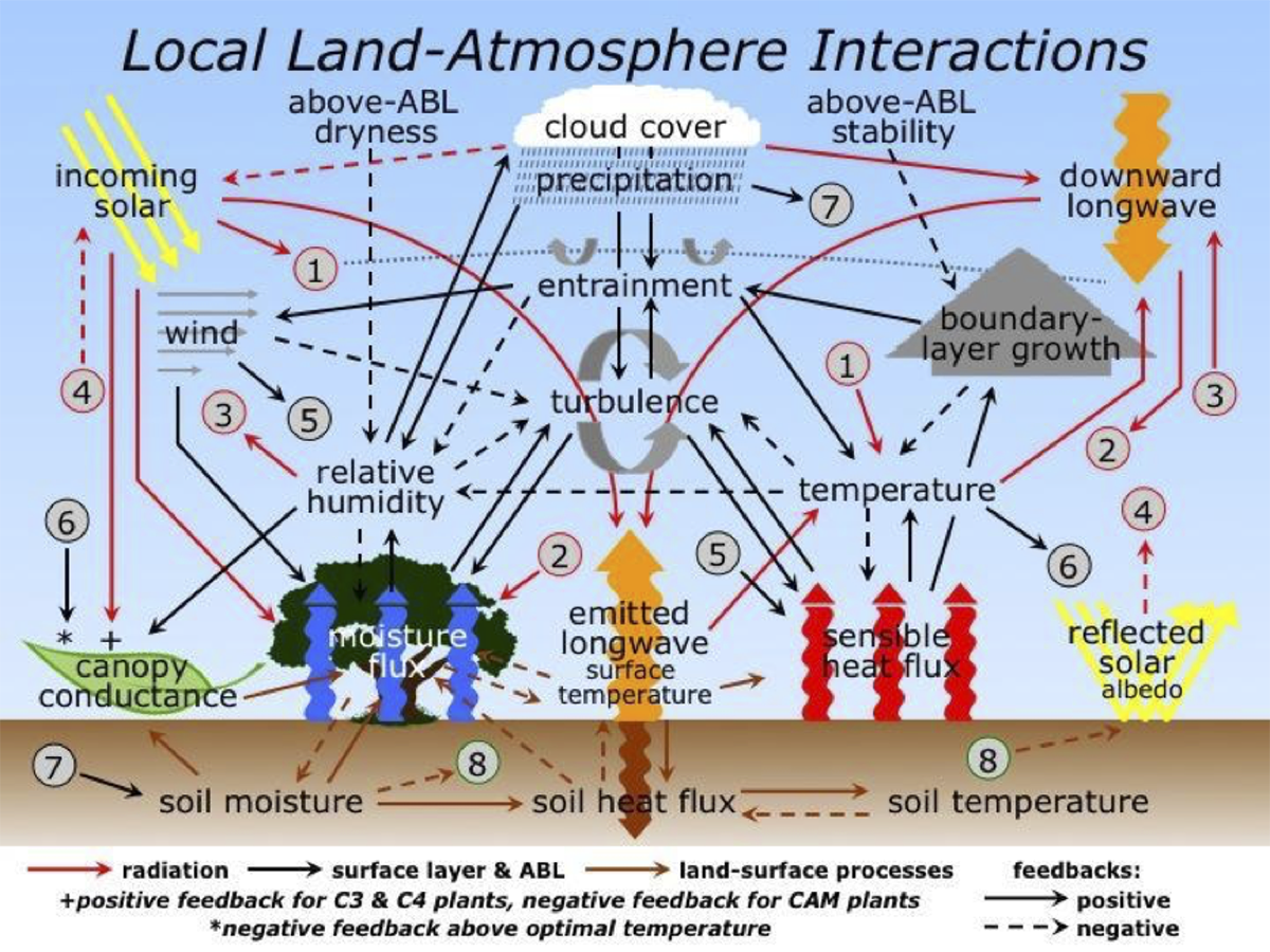
Earth system models connect the atmosphere, ocean, and land, and depend on proper representations of dynamics and physics, initial conditions, and interactions of these processes to predict future conditions. Standard meteorological variables are used to validate typical numerical weather prediction models but are gross measures of these countless interactions and limit their usefulness for guiding model improvement. Some fraction of error in these metrics can be the result of specific physical parameterizations, but it can be difficult to trace the source. One solution is to isolate these parameterizations – compare them with something measurable. These process-level metrics can help us begin to understand and then address the systematic biases in a given parameterization before we can consider the root causes of systematic biases in a more fully-coupled model.
Single Column Model (SCM) testing is part of the hierarchical model development approach by the Global Model Test Bed (GMTB) under the Developmental Testbed Center (DTC). DTC/GMTB is a joint effort between NCAR and NOAA/ESRL, in collaboration with their external research-to-operations partners, and led by personnel in NCAR/RAL/JNT and NOAA/ESRL/GSD. Single column models (SCMs) are an excellent way to evaluate the performance of a set of model physics because many physical processes primarily interact in the vertical, with horizontal transport by dynamics. Here, the model physical parameterizations are connected (as a column) and are provided with the necessary initial conditions and lateral forcing to investigate the evolution of the profile. SCM forcing may be from model, observational (e.g. from field programs) or idealized/synthetic data sets, to explore the response of the physics in different conditions, as well as to “stress test” parameterizations. In addition, computational resources required to run a SCM are orders of magnitude smaller than a fully-coupled model, and so may run in seconds on a laptop. SCMs with options to turn on and off various parameterizations, then allow for the examination of the interactions of those parameterizations, e.g. land plus surface-layer turbulence plus atmospheric boundary-layer.
The question to answer is, “do we obtain the same performance when the parameterizations are run separately as we do when they are coupled?” A model can be tuned to obtain some required level of performance, but the more complex the system, the more tuning may be accommodating a number of compensating errors, rather than making improvements to the model physics. What we are ultimately after is "getting the right answers for the right reasons," first testing a parameterization in isolation, then progressively adding parameterization interactions, up to a SCM. Using SCMs can enhance interactions with the Research-to-Operations (R2O) community, where they often work on physics development, but may not have their focus on or computer resources to do fully-coupled model runs, which could include data flow, data assimilation, model output post-processing, etc.
Note that at higher resolutions (model grid boxes that are on the order of 5-10 km or less), the evaluation of some physics (most notable convection and convective systems) requires at least a limited-area model to examine processes and identify systematic biases, where circulations are induced between grid boxes. This is a part of the hierarchy of model testing and development, where the follow-on steps are then regional, continental, and global-scale models, which have more traditional NWP metrics of performance. One must still get the physics right with process-level metrics of performance. We must “look under the hood” to see what is really going on if we are to make real improvements in the performance of Earth system and numerical weather prediction models.
